
In this tutorial, you will learn how to change the input shape tensor dimensions for fine-tuning using Keras. After going through this guide you’ll understand how to apply transfer learning to images with different image dimensions than what the CNN was originally trained on.
A few weeks ago I published a tutorial on transfer learning with Keras and deep learning — soon after the tutorial was published, I received a question from Francesca Maepa who asked the following:
Do you know of a good blog or tutorial that shows how to implement transfer learning on a dataset that has a smaller shape than the pre-trained model?
I created a really good pre-trained model, and would like to use some features for the pre-trained model and transfer them to a target domain that is missing certain feature training datasets and I’m not sure if I’m doing it right.
Francesca asks a great question.
Typically we think of Convolutional Neural Networks as accepting fixed size inputs (i.e., 224×224, 227×227, 299×299, etc.).
But what if you wanted to:
- Utilize a pre-trained network for transfer learning…
- …and then update the input shape dimensions to accept images with different dimensions than what the original network was trained on?
Why might you want to utilize different image dimensions?
There are two common reasons:
- Your input image dimensions are considerably smaller than what the CNN was trained on and increasing their size introduces too many artifacts and dramatically hurts loss/accuracy.
- Your images are high resolution and contain small objects that are hard to detect. Resizing to the original input dimensions of the CNN hurts accuracy and you postulate increasing resolution will help improve your model.
In these scenarios, you would wish to update the input shape dimensions of the CNN and then be able to perform transfer learning.
The question then becomes, is such an update possible?
Yes, in fact, it is.
Looking for the source code to this post?
Jump right to the downloads section.
Change input shape dimensions for fine-tuning with Keras
In the first part of this tutorial, we’ll discuss the concept of an input shape tensor and the role it plays with input image dimensions to a CNN.
From there we’ll discuss the example dataset we’ll be using in this blog post. I’ll then show you how to:
- Update the input image dimensions to pre-trained CNN using Keras.
- Fine-tune the updated CNN. Let’s get started!
What is an input shape tensor?
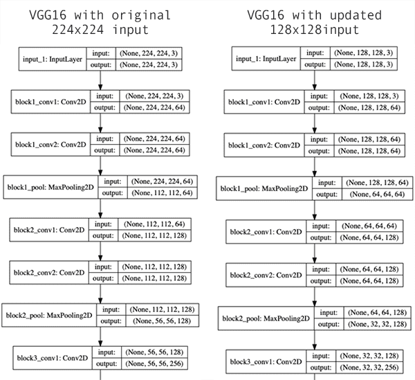
Figure 1: Convolutional Neural Networks built with Keras for deep learning have different input shape expectations. In this blog post, you’ll learn how to change input shape dimensions for fine-tuning with Keras.
When working with Keras and deep learning, you’ve probably either utilized or run into code that loads a pre-trained network via:
model = VGG16(weights="imagenet")
The code above is initializing the VGG16 architecture and then loading the weights for the model (pre-trained on ImageNet).
We would typically use this code when our project needs to classify input images that have class labels inside ImageNet (as this tutorial demonstrates).
When performing transfer learning or fine-tuning you may use the following code to leave off the fully-connected (FC) layer heads:
model = VGG16(weights="imagenet", include_top=False)
We’re still indicating that the pre-trained ImageNet weights should be used, but now we’re setting
include_top=False, indicating that the FC head should not be loaded.
This code would typically be utilized when you’re performing transfer learning either via feature extraction or fine-tuning.
Finally, we can update our code to include an input_tensor dimension:
model = VGG16(weights="imagenet", include_top=False,
	input_tensor=Input(shape=(224, 224, 3)))
We’re still loading VGG16 with weights pre-trained on ImageNet and we’re still leaving off the FC layer heads…but now we’re specifying an input shape of 224×224x3 (which are the input image dimensions that VGG16 was originally trained on, as seen in Figure 1, left).
That’s all fine and good — but what if we now wanted to fine-tune our model on 128×128px images?
That’s actually just a simple update to our model initialization:
model = VGG16(weights="imagenet", include_top=False,
	input_tensor=Input(shape=(128, 128, 3)))
Figure 1 (right) provides a visualization of the network updating the input tensor dimensions — notice how the input volume is now 128x128x3 (our updated, smaller dimensions) versus the previous 224x224x3 (the original, larger dimensions).
Updating the input shape dimensions of a CNN via Keras is that simple!
But there are a few caveats to look out for.
Can I make the input dimensions anything I want?

Figure 2: Updating a Keras CNN’s input shape is straightforward; however, there are a few caveats to take into consideration,
There are limits to how much you can update the image dimensions, both from an accuracy/loss perspective and from limitations of the network itself.
Consider the fact that CNNs reduce volume dimensions via two methods:
- Pooling (such as max-pooling in VGG16)
- Strided convolutions (such as in ResNet)
If your input image dimensions are too small then the CNN will naturally reduce volume dimensions during the forward propagation and then effectively “run out” of data.
In that case your input dimensions are too small.
I’ve included an error of what happens during that scenario below when, for example, when using 48×48 input images, I received this error message:
ValueError: Negative dimension size caused by subtracting 4 from 1 for 'average_pooling2d_1/AvgPool' (op: 'AvgPool') with input shapes: [?,1,1,512].
Notice how Keras is complaining that our volume is too small. You will encounter similar errors for other pre-trained networks as well. When you see this type of error, you know you need to increase your input image dimensions.
You can also make your input dimensions too large.
You won’t run into any errors per se, but you may see your network fail to obtain reasonable accuracy due to the fact that there are not enough layers in the network to:
- Learn robust, discriminative filters.
- Naturally reduce volume size via pooling or strided convolution.
If that happens, you have a few options:
- Explore other (pre-trained) network architectures that are trained on larger input dimensions.
- Tune your hyperparameters exhaustively, focusing first on learning rate.
- Add additional layers to the network. For VGG16 you’ll use 3×3 CONV layers and max-pooling. For ResNet you’ll include residual layers with strided convolution.
The final suggestion will require you to update the network architecture and then perform fine-tuning on the newly initialized layers.
To learn more about fine-tuning and and transfer learning, along with my tips, suggestions, and best practices when training networks, make sure you refer to my book, Deep Learning for Computer Vision with Python.
Our example dataset
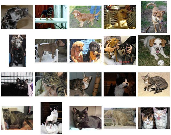
Figure 3: A subset of the Kaggle Dogs vs. Cats dataset is used for this Keras input shape example. Using a smaller dataset not only proves the point more quickly, but also allows just about any computer hardware to be used (i.e. no expensive GPU machine/instance necessary).
The dataset we’ll be using here today is a small subset of Kaggle’s Dogs vs. Cats dataset.
We also use this dataset inside Deep Learning for Computer Vision with Python to teach the fundamentals of training networks, ensuring that readers with either CPUs or GPUs can follow along and learn best practices when training models.
The dataset itself contains 2,000 images belonging to 2 classes (“cat” and dog”):
- Cat: 1,000 images
- Dog: 1,000 images
A visualization of the dataset can be seen in Figure 3 above.
In the remainder of this tutorial you’ll learn how to take this dataset and:
- Update the input shape dimensions for a pre-trained CNN.
- Fine-tune the CNN with the smaller image dimensions.
Installing necessary packages
All of today’s packages can be installed via pip.
I recommend that you create a Python virtual environment for today’s project, but it is not necessarily required. To learn how to create a virtual environment quickly and to install OpenCV into it, refer to my pip install opencv tutorial.
To install the packages for today’s project, just enter the following commands:
$ workon <env_name>
$ pip install opencv-contrib-python # includes numpy
$ pip install imutils
$ pip install matplotlib
$ pip install scikit-learn
$ pip install tensorflow # or tensorflow-gpu
$ pip install keras
Project structure
Go ahead and grab the code + dataset from the “Downloads“ section of today’s blog post.
Once you’ve extracted the .zip archive, you may inspect the project structure using the
treecommand:
$ tree --dirsfirst --filelimit 10
.
├── dogs_vs_cats_small
│   ├── cats [1000 entries]
│   └── dogs [1000 entries]
├── plot.png
└── train.py

3 directories, 2 files
Our dataset is contained within the
dogs_vs_cats_small/directory. The two subdirectories contain images of our classes. If you’re working with a different dataset be sure the structure is
<dataset>/<class_name>.
Today we’ll be reviewing the
train.pyscript. The training script generates
plot.pngcontaining our accuracy/loss curves.
Updating the input shape dimensions with Keras
It’s now time to update our input image dimensions with Keras and a pre-trained CNN.
Open up the
train.pyfile in your project structure and insert the following code:
# import the necessary packages
from keras.preprocessing.image import ImageDataGenerator
from keras.layers.pooling import AveragePooling2D
from keras.applications import VGG16
from keras.layers.core import Dropout
from keras.layers.core import Flatten
from keras.layers.core import Dense
from keras.layers import Input
from keras.models import Model
from keras.optimizers import Adam
from keras.utils import np_utils
from sklearn.preprocessing import LabelBinarizer
from sklearn.model_selection import train_test_split
from sklearn.metrics import classification_report
from imutils import paths
import matplotlib.pyplot as plt
import numpy as np
import argparse
import cv2
import os
Lines 2-20 import required packages:
keras
andsklearn
are for deep learning/machine learning. Be sure to refer to my extensive deep learning book, Deep Learning for Computer Vision with Python, to become more familiar with the classes and functions we use from these tools.paths
from imutils traverses a directory and enables us to list all images in a directory.matplotlib
will allow us to plot our training accuracy/loss history.numpy
is a Python package for numerical operations; one of the ways we’ll put it to work is for “mean subtraction”, a scaling/normalization technique.cv2
is OpenCV.argparse
will be used to read and parse command line arguments.
Let’s go ahead and parse the command line arguments now:
# construct the argument parser and parse the arguments
ap = argparse.ArgumentParser()
ap.add_argument("-d", "--dataset", required=True,
	help="path to input dataset")
ap.add_argument("-e", "--epochs", type=int, default=25,
	help="# of epochs to train our network for")
ap.add_argument("-p", "--plot", type=str, default="plot.png",
	help="path to output loss/accuracy plot")
args = vars(ap.parse_args())
Our script accepts three command line arguments via Lines 23-30:
--dataset
: The path to our input dataset. We’re using a condensed version of Dogs vs. Cats, but you could use other binary, 2-class datasets with little or no modification as well (provided they follow a similar structure).--epochs
: The number of times we’ll pass our data through the network during training; by default, we’ll train for25
epochs unless a different value is supplied.--plot
: The path to our output accuracy/loss plot. Unless otherwise specified, the file will be namedplot.png
and placed in the project directory. If you are conducting multiple experiments, be sure to give your plots a different name each time for future comparison purposes.
Next, we will load and preprocess our images:
# grab the list of images in our dataset directory, then initialize
# the list of data (i.e., images) and class images
print("[INFO] loading images...")
imagePaths = list(paths.list_images(args["dataset"]))
data = []
labels = []

# loop over the image paths
for imagePath in imagePaths:
	# extract the class label from the filename
	label = imagePath.split(os.path.sep)[-2]

	# load the image, swap color channels, and resize it to be a fixed
	# 128x128 pixels while ignoring aspect ratio
	image = cv2.imread(imagePath)
	image = cv2.cvtColor(image, cv2.COLOR_BGR2RGB)
	image = cv2.resize(image, (128, 128))

	# update the data and labels lists, respectively
	data.append(image)
	labels.append(label)
First, we grab our
imagePathson Line 35 and then initialize our
dataand
labels(Lines 36 and 37).
Lines 40-52 loop over the
imagePathswhile first extracting the labels. Each image is loaded, the color channels are swapped, and the image is resized. The images and labels are added to the
dataand
labelslists respectively.
VGG16 was trained on 224×224px images; however, I’d like to draw your attention to Line 48. Notice how we’ve resized our images to 128×128px. This resizing is an example of applying transfer learning on images with different dimensions.
Although Line 48 doesn’t fully answer Francesca Maepa’s question yet, we’re getting close.
Let’s go ahead and one-hot encode our labels as well as split our data:
# convert the data and labels to NumPy arrays
data = np.array(data)
labels = np.array(labels)

# perform one-hot encoding on the labels
lb = LabelBinarizer()
labels = lb.fit_transform(labels)
labels = np_utils.to_categorical(labels)

# partition the data into training and testing splits using 75% of
# the data for training and the remaining 25% for testing
(trainX, testX, trainY, testY) = train_test_split(data, labels,
	test_size=0.25, stratify=labels, random_state=42)
Lines 55 and 56 convert our
dataand
labelsto NumPy array format.
Then, Lines 59-61 perform one-hot encoding on our labels. Essentially, this process converts our two labels (“cat” and “dog”) to arrays indicating which label is active/hot. If a training image is representative of a dog, then the value would be
[0, 1]where “dog” is hot. Otherwise, for a “cat”, the value would be
[1, 0].
To reinforce the point, if for example, we had 5 classes of data, a one-hot encoded array may look like
[0, 0, 0, 1, 0]where the 4th element is hot indicating that the image is from the 4th class. For further details, please refer to Deep Learning for Computer Vision with Python.
Lines 65 and 66 mark 75% of our data for training and the remaining 25% for testing via the
train_test_splitfunction.
Let’s now initialize our data augmentation generator. We’ll also establish our ImageNet mean for mean subtraction:
# initialize the training data augmentation object
trainAug = ImageDataGenerator(
	rotation_range=30,
	zoom_range=0.15,
	width_shift_range=0.2,
	height_shift_range=0.2,
	shear_range=0.15,
	horizontal_flip=True,
	fill_mode="nearest")

# initialize the validation/testing data augmentation object (which
# we'll be adding mean subtraction to)
valAug = ImageDataGenerator()

# define the ImageNet mean subtraction (in RGB order) and set the
# the mean subtraction value for each of the data augmentation
# objects
mean = np.array([123.68, 116.779, 103.939], dtype="float32")
trainAug.mean = mean
valAug.mean = mean
Lines 69-76 initialize a data augmentation object for performing random manipulations on our input images during training.
Line 80 also takes advantage of the
ImageDataGeneratorclass for validation, but without any parameters — we won’t manipulate validation images with the exception of performing mean subtraction.
Both training and validation/testing generators will conduct mean subtraction. Mean subtraction is a scaling/normalization technique proven to increase accuracy. Line 85 contains the mean for each respective RGB channel while Lines 86 and 87 are then populated with the value. Later, our data generators will automatically perform the mean subtraction on our training/validation data.
Note: I’ve covered data augmentation in detail in this blog post as well as in the Practitioner Bundle of Deep Learning for Computer Vision with Python. Scaling and normalization techniques such as mean subtraction are covered in DL4CV as well.
We’re performing transfer learning with VGG16. Let’s initialize the base model now:
# load VGG16, ensuring the head FC layer sets are left off, while at
# the same time adjusting the size of the input image tensor to the
# network
baseModel = VGG16(weights="imagenet", include_top=False,
	input_tensor=Input(shape=(128, 128, 3)))

# show a summary of the base model
print("[INFO] summary for base model...")
print(baseModel.summary())
Lines 92 and 93 load
VGG16with an input shape dimension of 128×128 using 3 channels.
Remember, VGG16 was originally trained on 224×224 images — now we’re updating the input shape dimensions to handle 128×128 images.
Effectively, we have now fully answered Francesca Maepa’s question! We accomplished changing the input dimensions via two steps:
- We resized all of our input images to 128×128.
- Then we set the input
shape=(128, 128, 3)
.
Line 97 will print a model summary in our terminal so that we can inspect it. Alternatively, you may visualize the model graphically by studying Chapter 19 “Visualizing Network Architectures” of Deep Learning for Computer Vision with Python.
Since we’re performing transfer learning, the
include_topparameter is set to
False(Line 92) — we chopped off the head!
Now we’re going to perform surgery by erecting a new head and suturing it onto the CNN:
# construct the head of the model that will be placed on top of the
# the base model
headModel = baseModel.output
headModel = AveragePooling2D(pool_size=(4, 4))(headModel)
headModel = Flatten(name="flatten")(headModel)
headModel = Dense(128, activation="relu")(headModel)
headModel = Dropout(0.5)(headModel)
headModel = Dense(2, activation="softmax")(headModel)

# place the head FC model on top of the base model (this will become
# the actual model we will train)
model = Model(inputs=baseModel.input, outputs=headModel)

# loop over all layers in the base model and freeze them so they will
# *not* be updated during the first training process
for layer in baseModel.layers:
	layer.trainable = False
Line 101 takes the output from the
baseModeland sets it as input to the
headModel.
From there, Lines 102-106 construct the rest of the head.
The
baseModelis already initialized with ImageNet weights per Line 92. On Lines 114 and 115, we set the base layers in VGG16 as not trainable (i.e., they will not be updated during the backpropagation phase). Be sure to read my previous fine-tuning tutorial for further explanation.
We’re now ready to compile and train the model with our data:
# compile our model (this needs to be done after our setting our
# layers to being non-trainable)
print("[INFO] compiling model...")
opt = Adam(lr=1e-4)
model.compile(loss="binary_crossentropy", optimizer=opt,
	metrics=["accuracy"])

# train the head of the network for a few epochs (all other layers
# are frozen) -- this will allow the new FC layers to start to become
# initialized with actual "learned" values versus pure random
print("[INFO] training head...")
H = model.fit_generator(
	trainAug.flow(trainX, trainY, batch_size=32),
	steps_per_epoch=len(trainX) // 32,
	validation_data=valAug.flow(testX, testY),
	validation_steps=len(testX) // 32,
	epochs=args["epochs"])
Our
modelis compiled with the
Adamoptimizer and a
1e-4learning rate (Lines 120-122).
We use
"binary_crossentropy"for 2-class classification. If you have more than two classes of data, be sure to use
"categorical_crossentropy".
Lines 128-133 then train our transfer learning network. Our training and validation generators are put to work in the process.
Upon training completion, we’ll evaluate the network and plot the training history:
# evaluate the network
print("[INFO] evaluating network...")
predictions = model.predict(testX, batch_size=32)
print(classification_report(testY.argmax(axis=1),
	predictions.argmax(axis=1), target_names=lb.classes_))

# plot the training loss and accuracy
N = args["epochs"]
plt.style.use("ggplot")
plt.figure()
plt.plot(np.arange(0, N), H.history["loss"], label="train_loss")
plt.plot(np.arange(0, N), H.history["val_loss"], label="val_loss")
plt.plot(np.arange(0, N), H.history["acc"], label="train_acc")
plt.plot(np.arange(0, N), H.history["val_acc"], label="val_acc")
plt.title("Training Loss and Accuracy on Dataset")
plt.xlabel("Epoch #")
plt.ylabel("Loss/Accuracy")
plt.legend(loc="lower left")
plt.savefig(args["plot"])
Lines 137-139 evaluate our
modeland print a classification report for statistical analysis.
We then employ
matplotlibto plot our accuracy and loss history during training (Lines 142-152). The plot figure is saved to disk via Line 153.
Fine-tuning a CNN using the updated input dimensions
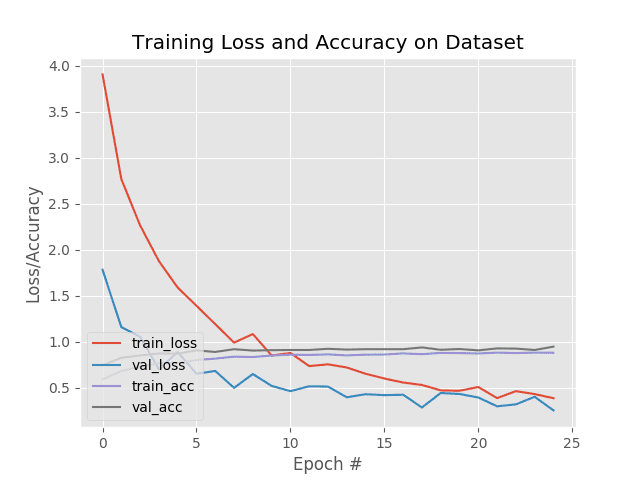
Figure 4: Changing Keras input shape dimensions for fine-tuning produced the following accuracy/loss training plot.
To fine-tune our CNN using the updated input dimensions first make sure you’ve used the “Downloads” section of this guide to download the (1) source code and (2) example dataset.
From there, open up a terminal and execute the following command:
$ python train.py --dataset dogs_vs_cats_small --epochs 25
Using TensorFlow backend.
[INFO] loading images...
[INFO] summary for base model...
_________________________________________________________________
Layer (type)                 Output Shape              Param #
=================================================================
input_1 (InputLayer)         (None, 128, 128, 3)       0
_________________________________________________________________
block1_conv1 (Conv2D)        (None, 128, 128, 64)      1792
_________________________________________________________________
block1_conv2 (Conv2D)        (None, 128, 128, 64)      36928
_________________________________________________________________
block1_pool (MaxPooling2D)   (None, 64, 64, 64)        0
_________________________________________________________________
block2_conv1 (Conv2D)        (None, 64, 64, 128)       73856
_________________________________________________________________
block2_conv2 (Conv2D)        (None, 64, 64, 128)       147584
_________________________________________________________________
block2_pool (MaxPooling2D)   (None, 32, 32, 128)       0
_________________________________________________________________
block3_conv1 (Conv2D)        (None, 32, 32, 256)       295168
_________________________________________________________________
block3_conv2 (Conv2D)        (None, 32, 32, 256)       590080
_________________________________________________________________
block3_conv3 (Conv2D)        (None, 32, 32, 256)       590080
_________________________________________________________________
block3_pool (MaxPooling2D)   (None, 16, 16, 256)       0
_________________________________________________________________
block4_conv1 (Conv2D)        (None, 16, 16, 512)       1180160
_________________________________________________________________
block4_conv2 (Conv2D)        (None, 16, 16, 512)       2359808
_________________________________________________________________
block4_conv3 (Conv2D)        (None, 16, 16, 512)       2359808
_________________________________________________________________
block4_pool (MaxPooling2D)   (None, 8, 8, 512)         0
_________________________________________________________________
block5_conv1 (Conv2D)        (None, 8, 8, 512)         2359808
_________________________________________________________________
block5_conv2 (Conv2D)        (None, 8, 8, 512)         2359808
_________________________________________________________________
block5_conv3 (Conv2D)        (None, 8, 8, 512)         2359808
_________________________________________________________________
block5_pool (MaxPooling2D)   (None, 4, 4, 512)         0
=================================================================
Total params: 14,714,688
Trainable params: 14,714,688
Non-trainable params: 0
Our first set of output shows our updated input shape dimensions.
Notice how our
input_1(i.e., the
InputLayer) has input dimensions of 128x128x3 versus the normal 224x224x3 for VGG16.
The input image will then forward propagate through the network until the final
MaxPooling2Dlayer (i.e.,
block5_pool).
At this point, our output volume has dimensions of 4x4x512 (for reference, VGG16 with a 224x224x3 input volume would have the shape 7x7x512 after this layer).
Note: If your input image dimensions are too small then you risk the model, effectively, reducing the tensor volume into “nothing” and then running out of data, leading to an error. See the “Can I make the input dimensions anything I want?” section of this post for more details.
We then flatten that volume and apply the FC layers from the
headModel, ultimately leading to our final classification.
Once our model is constructed we can then fine-tune it:
[INFO] compiling model...
[INFO] training head...
Epoch 1/25
46/46 [==============================] - 9s 199ms/step - loss: 3.9048 - acc: 0.5897 - val_loss: 1.7824 - val_acc: 0.7438
Epoch 2/25
46/46 [==============================] - 8s 182ms/step - loss: 2.7716 - acc: 0.6815 - val_loss: 1.1589 - val_acc: 0.8248
Epoch 3/25
46/46 [==============================] - 6s 130ms/step - loss: 2.2621 - acc: 0.7312 - val_loss: 1.0531 - val_acc: 0.8504
Epoch 4/25
46/46 [==============================] - 6s 130ms/step - loss: 1.8732 - acc: 0.7665 - val_loss: 0.6999 - val_acc: 0.8718
Epoch 5/25
46/46 [==============================] - 6s 130ms/step - loss: 1.5874 - acc: 0.7684 - val_loss: 0.8887 - val_acc: 0.8697
...
Epoch 21/25
46/46 [==============================] - 6s 130ms/step - loss: 0.5067 - acc: 0.8722 - val_loss: 0.3941 - val_acc: 0.9060
Epoch 22/25
46/46 [==============================] - 6s 131ms/step - loss: 0.3869 - acc: 0.8822 - val_loss: 0.2982 - val_acc: 0.9274
Epoch 23/25
46/46 [==============================] - 6s 131ms/step - loss: 0.4629 - acc: 0.8767 - val_loss: 0.3193 - val_acc: 0.9252
Epoch 24/25
46/46 [==============================] - 6s 130ms/step - loss: 0.4304 - acc: 0.8822 - val_loss: 0.4016 - val_acc: 0.9103
Epoch 25/25
46/46 [==============================] - 6s 130ms/step - loss: 0.3874 - acc: 0.8800 - val_loss: 0.2538 - val_acc: 0.9466
[INFO] evaluating network...
              precision    recall  f1-score   support

        cats       0.94      0.92      0.93       250
        dogs       0.92      0.94      0.93       250

   micro avg       0.93      0.93      0.93       500
   macro avg       0.93      0.93      0.93       500
weighted avg       0.93      0.93      0.93       500
At the end of fine-tuning we see that our model has obtained 93% accuracy, respectable given our small image dataset.
As Figure 4 demonstrates, our training is also quite stable as well with no signs of overfitting.
More importantly, you now know how to change the input image shape dimensions of a pre-trained network and then apply feature extraction/fine-tuning using Keras!
Be sure to use this tutorial as a template for whenever you need to apply transfer learning to a pre-trained network with different image dimensions than what it was originally trained on.
Summary
In this tutorial, you learned how to change input shape dimensions for fine-tuning with Keras.
We typically perform such an operation when we want to apply transfer learning, including both feature extraction and fine-tuning.
Using the methods in this guide, you can update your input image dimensions for your pre-trained CNN and then perform transfer learning; however, there are two caveats you need to look out for:
- If your input images are too small, Keras will error out.
- If your input images are too large, you may not obtain your desired accuracy.
Be sure to refer to the “Can I make the input dimensions anything I want?” section of this post for more details on these caveats, including suggestions on how to solve them.
I hope you enjoyed this tutorial!
To download the source code to this post, and be notified when future tutorials are published here on PyImageSearch, just enter your email address in the form below!
Downloads:
The post Change input shape dimensions for fine-tuning with Keras appeared first on PyImageSearch.