Quantcast
Channel: deep learning Archives - PyImageSearch
Viewing all 277 articles
Browse latest View live

Adversarial images and attacks with Keras and TensorFlow

$
0
0

In this tutorial, you will learn how to break deep learning models using image-based adversarial attacks. We will implement our adversarial attacks using the Keras and TensorFlow deep learning libraries.

Imagine it’s twenty years from now. Nearly all cars and trucks on the road have been replaced with autonomous vehicles, powered by Artificial Intelligence, deep learning, and computer vision — every turn, lane switch, acceleration, and brake is powered by a deep neural network.

Now, imagine you’re on the highway. You’re sitting in the “driver’s seat” (is it really a “driver’s seat” if the car is doing the driving?) while your spouse is in the passenger seat, and your kids are in the back.

Looking ahead, you see a large sticker plastered on the lane your car is driving in. It looks innocent enough. It’s just a big print of the graffiti artist Banksy’s popular Girl with Balloon work. Some high school kids probably just put it there as part of a weird dare/practical joke.

Figure 1: Performing an adversarial attack requires taking an input image (left), purposely perturbing it with a noise vector (middle), which forces the network to misclassify the input image, ultimately resulting in an incorrect classification, potentially with major consequences (right).

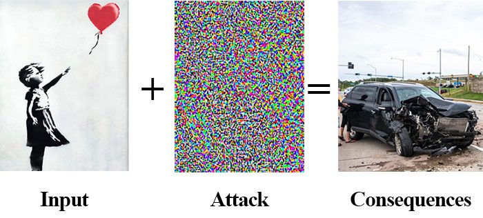
A split second later, your car reacts by violently breaking hard and then switching lanes as if the large art print plastered on the road is a human, an animal, or another vehicle. You’re jerked so hard that you feel the whiplash. Your spouse screams while Cheerios from your kid in the backseat rocket forward, hitting the windshield and bouncing all over the center console.

You and your family are safe … but it could have been a lot worse.

What happened? Why did your self-driving car react that way? Was it some sort of weird “bug” in the code/software your car is running?

The answer is that the deep neural network powering the “sight” component of your vehicle just saw an adversarial image.

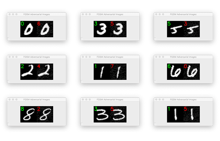
Adversarial images are:

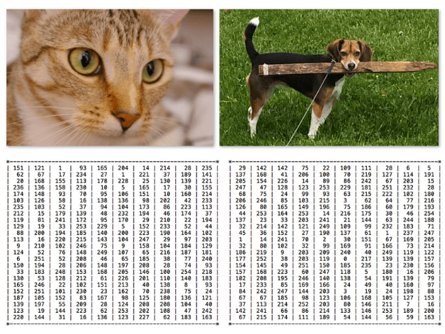
  1. Images that have pixels purposely and intentionally perturbed to confuse and deceive models …
  2. … but at the same time, look harmless and innocent to humans.

These images cause deep neural networks to purposely make incorrect predictions. Adversarial images are perturbed in such a way that the model is unable to correctly classify them.

In fact, it may be impossible for humans to visually identify a normal image from one that has been visually perturbed for an adversarial attack — essentially, the two images will appear identical to the human eye.

While not an exact (or correct) comparison, I like to explain adversarial attacks in the context of image steganography. Using steganography algorithms, we can embed data (such as plaintext messages) in an image without distorting the appearance of the image itself. This image can be innocently transmitted to the receiver, who can then extract the hidden message from the image.

Similarly, adversarial attacks embed a message in an input image — but instead of a plaintext message meant for human consumption, an adversarial attack instead embeds a noise vector in the input image. This noise vector is purposely constructed to fool and confuse deep learning models.

But how do adversarial attacks work? And how can we defend against them?

This tutorial, along with the rest of the posts in this series, will cover that exact same question.

To learn how to break deep learning models with adversarial attacks and images using Keras/TensorFlow, just keep reading.

Looking for the source code to this post?

Jump Right To The Downloads Section

Adversarial images and attacks with Keras and TensorFlow

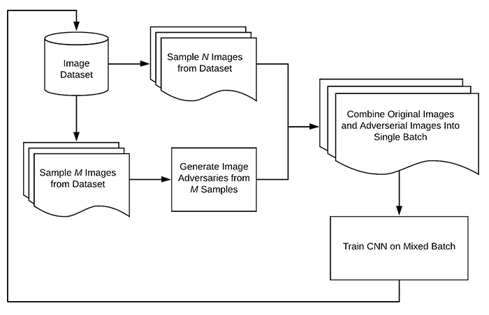
In the first part of this tutorial, we’ll discuss what adversarial attacks are and how they impact deep learning models.

From there, we’ll implement three separate Python scripts:

  1. The first one will be a helper utility used to load and parse class labels from the ImageNet dataset.
  2. Our next Python script will perform basic image classification using ResNet, pre-trained on the ImageNet dataset (thereby demonstrating “standard” image classification).
  3. The final Python script will perform an adversarial attack and construct an adversarial image that purposely confuses our ResNet model, even though the two images look identical to the human eye.

Let’s get started!

What are adversarial images and adversarial attacks? And how to they impact deep learning models?

Figure 2: When performing an adversarial attack, we present an input image (left) to our neural network. We then use gradient descent to construct the noise vector (middle). This noise vector is added to the input image, resulting in a misclassification (right). (Image source: Figure 1 of Explaining and Harnessing Adversarial Examples)

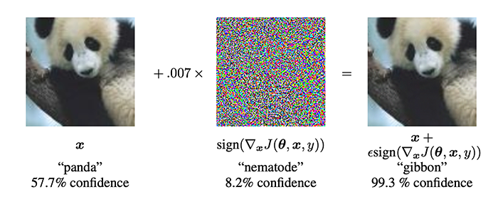
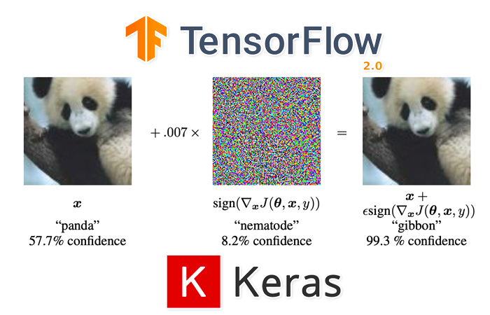
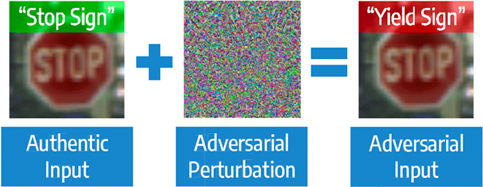
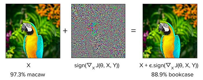
In 2014, Goodfellow et al. published a paper entitled Explaining and Harnessing Adversarial Examples, which showed an intriguing property of deep neural networks — it’s possible to purposely perturb an input image such that the neural network misclassifies it. This type of perturbation is called an adversarial attack.

The classic example of an adversarial attack can be seen in Figure 2 above. On the left, we have our input image which our neural network correctly classifies as “panda” with 57.7% confidence.

In the middle, we have a noise vector, which to the human eye, appears to be random. However, it’s far from random.

Instead, the pixels in noise vector are “equal to the sign of the elements of the gradient of the cost function with the respect to the input image” (Goodfellow et al.).

We then add this noise vector to the input image, which produces the output (right) in Figure 2. To us, this image appears identical to the input; however, our neural network now classifies the image as a “gibbon” (a small ape, similar to a monkey) with 99.7% confidence.

Creepy, right?

A brief history of adversarial attacks and images

Figure 3: A timeline of adversarial machine learning and security of deep neural network publications (Image source: Figure 8 of Can Machine Learning Be Secure?)

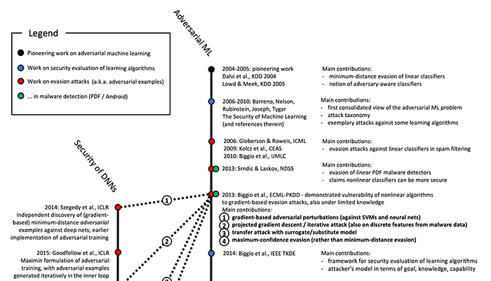
Adversarial machine learning is not a new field, nor are these attacks specific to deep neural networks. In 2006, Barreno et al. published a paper entitled Can Machine Learning Be Secure? This paper discussed adversarial attacks, including proposed defenses against them.

Back in 2006, the top state-of-the-art machine learning models included Support Vector Machines (SVMs) and Random Forests (RFs) — it’s been shown that both these types of models are susceptible to adversarial attacks.

With the rise in popularity of deep neural networks starting in 2012, it was hoped that these highly non-linear models would be less susceptible to attacks; however, Goodfellow et al. (among others) dashed these hopes.

It turns out that deep neural networks are susceptible to adversarial attacks, just like their predecessors.

For more information on the history of adversarial attacks, I recommend reading Biggio and Roli’s excellent 2017 paper, Wild Patterns: Ten Years After the Rise of Adversarial Machine Learning.

Why are adversarial attacks and images a problem?

Figure 4: Why are adversarial attacks such a problem? Why should we be concerned? (image source)

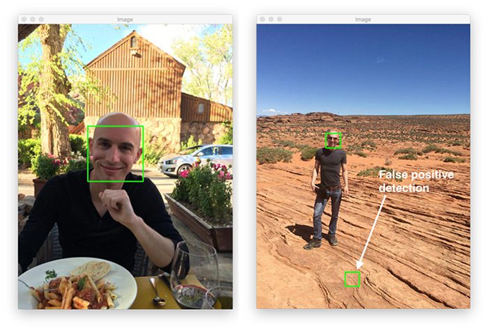
The example at the top of this tutorial outlined why adversarial attacks could cause massive damage to health, life, and property.

Examples with less severe consequences could be a group of hackers identifies that a specific model is being used by Google for spam filtering in Gmail, or a given model is being used by Facebook to automatically detect pornography in their NSFW filter.

If these hackers wanted to flood Gmail users with emails that bypass Gmail’s spam filters, or upload massive amounts of pornography to Facebook that bypasses their NSFW filters, they could theoretically do so.

These are all examples of adversarial attacks with less consequences.

An adversarial attack in a scenario with higher consequences could include hacker-terrorists identifying that a specific deep neural network is being used for nearly all self-driving cars in the world (imagine if Tesla had a monopoly on the market and was the only self-driving car producer).

Adversarial images could then be strategically placed along roads and highways, causing massive pileups, property damage, and even injury/death to passengers in the vehicles.

The limit to adversarial attacks is only limited by your imagination, your knowledge of a given model, and how much access you have to the model itself.

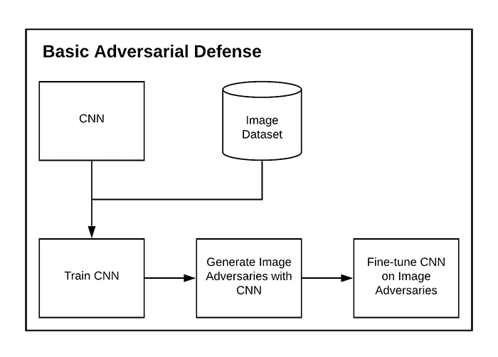
Can we defend against adversarial attacks?

The good news is that we can help reduce the impact of adversarial attacks (but not necessarily eliminate them completely).

That topic won’t be covered in today’s tutorial, but will be covered in a future tutorial on PyImageSearch.

Configuring your development environment

To configure your system for this tutorial, I recommend following either of these tutorials:

Either tutorial will help you configure your system with all the necessary software for this blog post in a convenient Python virtual environment.

That said, are you:

  • Short on time?
  • Learning on your employer’s administratively locked laptop?
  • Wanting to skip the hassle of fighting with package managers, bash/ZSH profiles, and virtual environments?
  • Ready to run the code right now (and experiment with it to your heart’s content)?

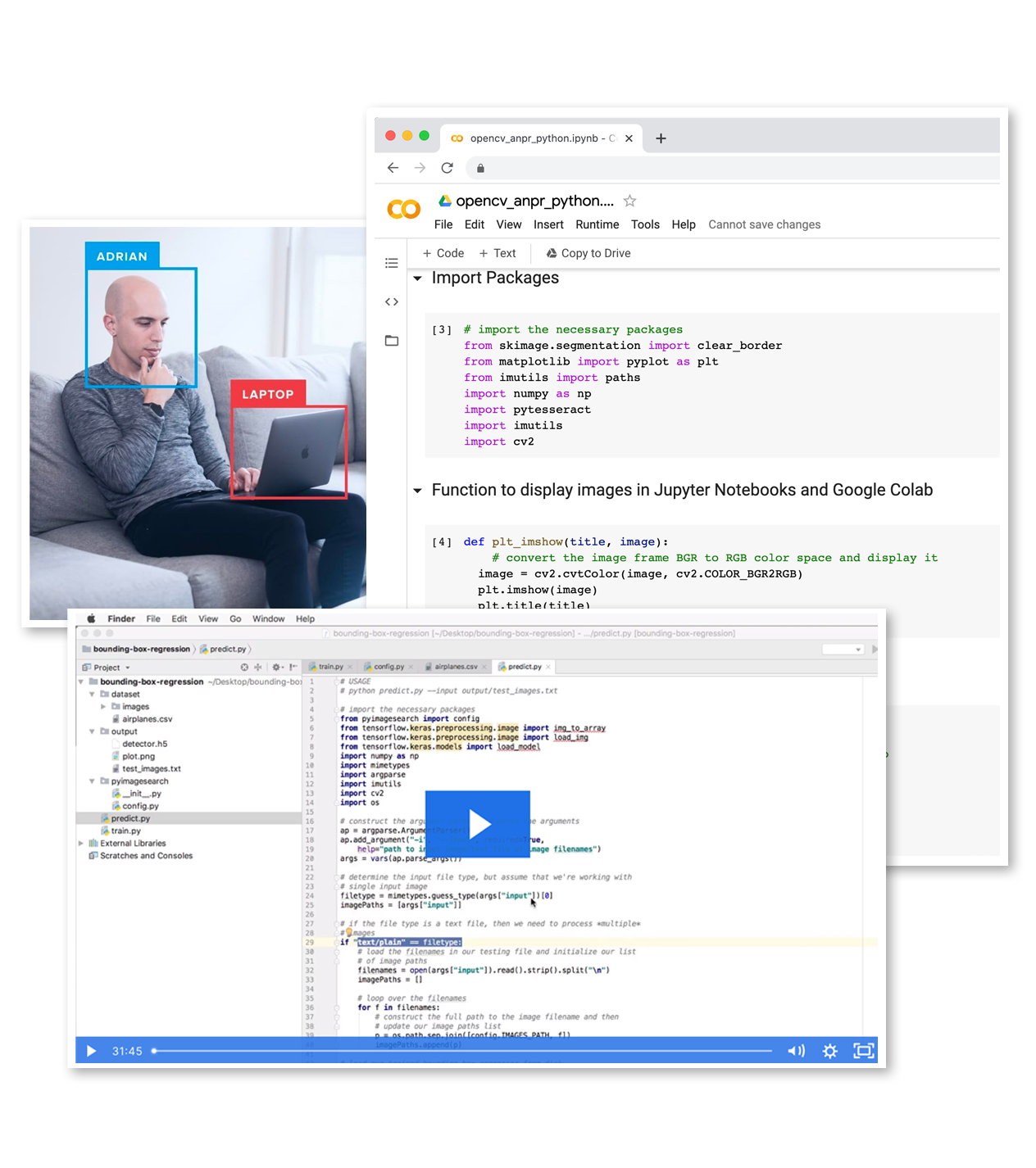
Then join PyImageSearch Plus today! Gain access to PyImageSearch tutorial Jupyter Notebooks that run on Google’s Colab ecosystem in your browser — no installation required!

Project structure

Start by using the “Downloads” section of this tutorial to download the source code and example images. From there, let’s inspect our project directory structure.

$ tree --dirsfirst
.
├── pyimagesearch
│   ├── __init__.py
│   ├── imagenet_class_index.json
│   └── utils.py
├── adversarial.png
├── generate_basic_adversary.py
├── pig.jpg
└── predict_normal.py

1 directory, 7 files

Inside the pyimagesearch module, we have two files:

  1. imagenet_class_index.json: A JSON file, which maps ImageNet class labels to human-readable strings. We’ll be using this JSON file to determine the integer index for a particular class label — this integer index will aid us when we construct our adversarial image attack.
  2. utils.py: Contains a simple Python helper function used to load and parse the imagenet_class_index.json.

We then have two Python scripts that we’ll be reviewing today:

  1. predict_normal.py: Accepts an input image (pig.jpg), loads our ResNet50 model, and classifies it. The output of this script will be the ImageNet class label index of the predicted class label.
  2. generate_basic_adversary.py: Using the output of our predict_normal.py script, we’ll construct an adversarial attack that is able to fool ResNet. The output of this script (adversarial.png) will be saved to disk.

Ready to implement your first adversarial attack with Keras and TensorFlow?

Let’s dive in.

Our ImageNet class label/index helper utility

Before we can perform either normal image classification or classification with an image perturbed via an adversarial attack, we first need to create a Python helper function used to load and parse the class labels of the ImageNet dataset.

We have provided a JSON file that contains the ImageNet class label indexes, identifiers, and human-readable strings inside the imagenet_class_index.json file in the pyimagesearch module of our project directory structure.

I’ve included the first few lines of this JSON file below:

{
  "0": [
    "n01440764",
    "tench"
  ],
  "1": [
    "n01443537",
    "goldfish"
  ],
  "2": [
    "n01484850",
    "great_white_shark"
  ],
  "3": [
    "n01491361",
    "tiger_shark"
  ],
...
"106": [
    "n01883070",
    "wombat"
  ],
...

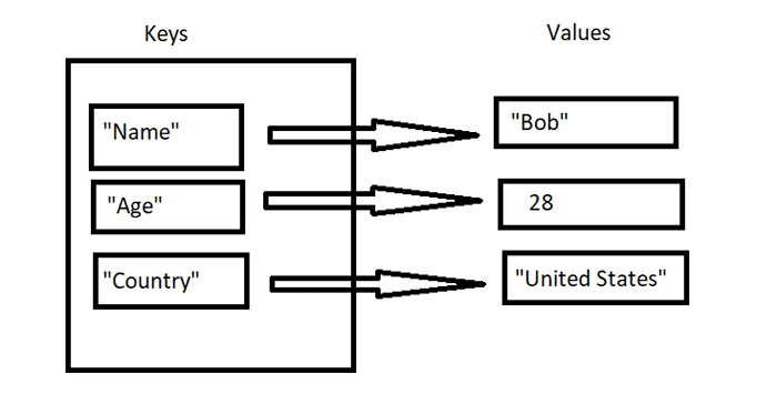
Here you can see that the file is a dictionary. The key to the dictionary is the integer class label index, while the value is 2-tuple consisting of:

  1. The ImageNet unique identifier for the label
  2. The human-readable class label

Our goal is to implement a Python function that will parse the JSON file by:

  1. Accepting an input class label
  2. Returning the integer class label index of the corresponding label

Essentially, we are inverting the key/value relationship in the imagenet_class_index.json file.

Let’s start implementing our helper function now.

Open up the utils.py file in the pyimagesearch module, and insert the following code:

# import necessary packages
import json
import os

def get_class_idx(label):
	# build the path to the ImageNet class label mappings file
	labelPath = os.path.join(os.path.dirname(__file__),
		"imagenet_class_index.json")

Lines 2 and 3 import our required Python packages. We’ll be using the json Python module to load our JSON file, while the os package will be used to construct file paths, agnostic of which operating system you are using.

We then define our get_class_idx helper function. The goal of this function is to accept an input class label and then obtain the integer index of the prediction (i.e., which index out of the 1,000 class labels that a model trained on ImageNet would be able to predict).

Line 7 constructs the path to the imagenet_class_index.json, which lives inside the pyimagesearch module.

Let’s load the contents of that JSON file now:

	# open the ImageNet class mappings file and load the mappings as
	# a dictionary with the human-readable class label as the key and
	# the integer index as the value
	with open(labelPath) as f:
		imageNetClasses = {labels[1]: int(idx) for (idx, labels) in
			json.load(f).items()}

	# check to see if the input class label has a corresponding
	# integer index value, and if so return it; otherwise return
	# a None-type value
	return imageNetClasses.get(label, None)

Lines 13-15 open the labelPath file and proceed to invert the key/value relationship such that the key is the human-readable label string and the value is the integer index that corresponds to that label.

In order to obtain the integer index for the input label, we make a call to the .get method of the imageNetClasses dictionary (Line 20) — this call will return either:

  • The integer index of the label (if it exists in the dictionary)
  • And if the label does not exist in imageNetClasses, it will return None

This value is then returned to the calling function.

Let’s put our get_class_idx helper function to work in the following section.

Normal image classification without adversarial attacks using Keras and TensorFlow

With our ImageNet class label/index helper function implemented, let’s first create an image classification script that performs basic classification with no adversarial attacks.

This script will demonstrate that our ResNet model is performing as we would it expect it to (i.e., making correct predictions). Later in this tutorial, you’ll discover how to construct an adversarial image such that it confuses ResNet.

Let’s get started with our basic image classification script — open up the predict_normal.py file in your project directory structure, and insert the following code:

# import necessary packages
from pyimagesearch.utils import get_class_idx
from tensorflow.keras.applications import ResNet50
from tensorflow.keras.applications.resnet50 import decode_predictions
from tensorflow.keras.applications.resnet50 import preprocess_input
import numpy as np
import argparse
import imutils
import cv2

We import our required Python packages on Lines 2-9. These will all look fairly standard to you if you’ve ever worked with Keras, TensorFlow, and OpenCV before.

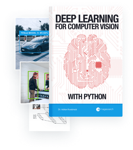
That said, if you are new to Keras and TensorFlow, I strongly encourage you to read my Keras Tutorial: How to get started with Keras, Deep Learning, and Python guide. Additionally, you may want to read my book Deep Learning for Computer Vision with Python to obtain a deeper understanding of how to train your own custom neural networks.

With all that said, take notice of Line 2, where we import our get_class_idx function, which we defined in the previous section — this function will allow us to obtain the integer index of the top predicted label from our ResNet50 model.

Let’s move on to defining our preprocess_image helper function:

def preprocess_image(image):
	# swap color channels, preprocess the image, and add in a batch
	# dimension
	image = cv2.cvtColor(image, cv2.COLOR_BGR2RGB)
	image = preprocess_input(image)
	image = cv2.resize(image, (224, 224))
	image = np.expand_dims(image, axis=0)

	# return the preprocessed image
	return image

The preprocess_image method accepts a single required argument, the image that we wish to preprocess.

We preprocess the image by:

  1. Swapping the image from BGR to RGB channel ordering
  2. Calling the preprocess_input image function, which performs ResNet50-specific preprocessing and scaling
  3. Resizing the image to 224×224
  4. Adding in a batch dimension

The preprocessed image is then returned to the calling function.

Next, let’s parse our command line arguments:

# construct the argument parser and parse the arguments
ap = argparse.ArgumentParser()
ap.add_argument("-i", "--image", required=True,
	help="path to input image")
args = vars(ap.parse_args())

We only need a single command line argument here, --image, which is the path to our input image residing on disk.

If you’ve never worked with command line arguments and argparse before, I suggest you read the following tutorial.

Let’s now load our input image from disk and preprocess it:

# load image from disk and make a clone for annotation
print("[INFO] loading image...")
image = cv2.imread(args["image"])
output = image.copy()

# preprocess the input image
output = imutils.resize(output, width=400)
preprocessedImage = preprocess_image(image)

A call to cv2.imread loads our input image from disk. We clone it on Line 31 so we can later draw on it/annotate it with the final output class label prediction.

We resize the output image to have a width of 400 pixels, such that it fits on our screen. We also call our preprocess_image function on the input image to prepare it for classification by ResNet.

With our image preprocessed, we can load ResNet and classify the image:

# load the pre-trained ResNet50 model
print("[INFO] loading pre-trained ResNet50 model...")
model = ResNet50(weights="imagenet")

# make predictions on the input image and parse the top-3 predictions
print("[INFO] making predictions...")
predictions = model.predict(preprocessedImage)
predictions = decode_predictions(predictions, top=3)[0]

On Line 39 we load ResNet from disk with weights pre-trained on the ImageNet dataset.

Lines 43 and 44 make predictions on our pre-procssed image, which we then decode using the decode_predictions helper function in Keras/TensorFlow.

Let’s now loop over the top-3 predictions from the network and display the class labels:

# loop over the top three predictions
for (i, (imagenetID, label, prob)) in enumerate(predictions):
	# print the ImageNet class label ID of the top prediction to our
	# terminal (we'll need this label for our next script which will
	# perform the actual adversarial attack)
	if i == 0:
		print("[INFO] {} => {}".format(label, get_class_idx(label)))

	# display the prediction to our screen
	print("[INFO] {}. {}: {:.2f}%".format(i + 1, label, prob * 100))

Line 47 begins a loop over the top-3 predictions.

If this is the first prediction (i.e., the top-1 prediction), we display the human-readable label to our terminal and then look up the ImageNet integer index of the corresponding label using our get_class_idx function.

We also display the top-3 labels and corresponding probability to our terminal.

The final step is to draw the top-1 prediction on the output image:

# draw the top-most predicted label on the image along with the
# confidence score
text = "{}: {:.2f}%".format(predictions[0][1],
	predictions[0][2] * 100)
cv2.putText(output, text, (3, 20), cv2.FONT_HERSHEY_SIMPLEX, 0.8,
	(0, 255, 0), 2)

# show the output image
cv2.imshow("Output", output)
cv2.waitKey(0)

The output image is displayed to our terminal until the window opened by OpenCV is clicked on and a key pressed.

Non-adversarial image classification results

We are now ready to perform basic image classification (i.e., no adversarial attack) with ResNet.

Start by using the “Downloads” section of this tutorial to download the source code and example images.

From there, open up a terminal and execute the following command:

$ python predict_normal.py --image pig.jpg
[INFO] loading image...
[INFO] loading pre-trained ResNet50 model...
[INFO] making predictions...
[INFO] hog => 341
[INFO] 1. hog: 99.97%
[INFO] 2. wild_boar: 0.03%
[INFO] 3. piggy_bank: 0.00%
Figure 5: Our pre-trained ResNet model is able to correctly classify this image as “hog”.

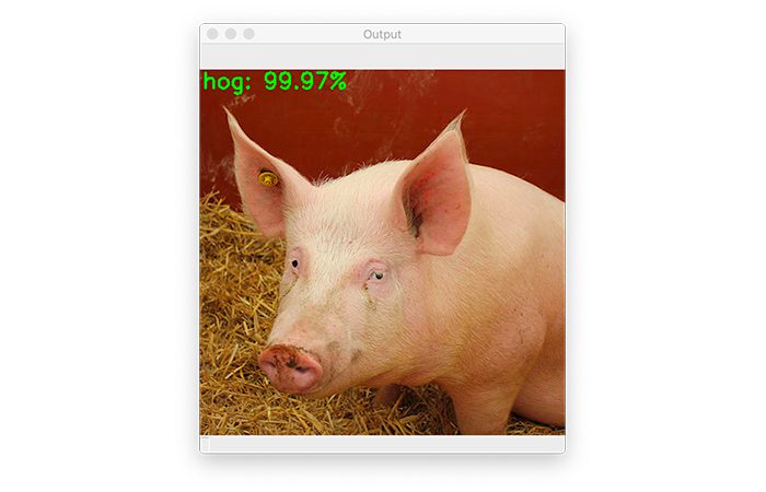
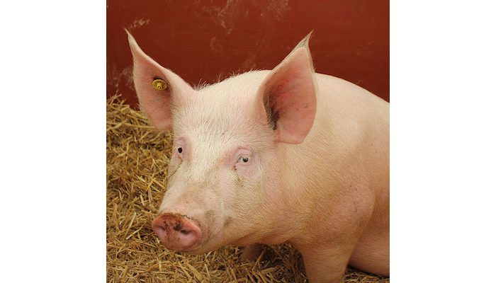
Here you can see that we have classified an input image of a pig, with 99.97% confidence.

Additionally, take note of the “hog” ImageNet label ID (341) — we’ll be using this class label ID in the next section, where we will perform an adversarial attack on the hog input image.

Implementing adversarial images and attacks with Keras and TensorFlow

We will now learn how to implement adversarial attacks with Keras and TensorFlow.

Open up the generate_basic_adversary.py file in our project directory structure, and insert the following code:

# import necessary packages
from tensorflow.keras.optimizers import Adam
from tensorflow.keras.applications import ResNet50
from tensorflow.keras.losses import SparseCategoricalCrossentropy
from tensorflow.keras.applications.resnet50 import decode_predictions
from tensorflow.keras.applications.resnet50 import preprocess_input
import tensorflow as tf
import numpy as np
import argparse
import cv2

We start by importing our required Python packages on Lines 2-10. You’ll notice that we are once again using the ResNet50 architecture with its corresponding preprocess_input function (for preprocessing/scaling input images) and decode_predictions utility to decode output predictions and display the human-readable ImageNet labels.

The SparseCategoricalCrossentropy computes the categorical cross-entropy loss between the labels and predictions. By using the sparse version implementation of categorical cross-entropy, we do not have to explicitly one-hot encode our class labels like we would if we were using scikit-learn’s LabelBinarizer or Keras/TensorFlow’s to_categorical utility.

Just like we had a preprocess_image utility in our predict_normal.py script, we also need one for this script as well:

def preprocess_image(image):
	# swap color channels, resize the input image, and add a batch
	# dimension
	image = cv2.cvtColor(image, cv2.COLOR_BGR2RGB)
	image = cv2.resize(image, (224, 224))
	image = np.expand_dims(image, axis=0)

	# return the preprocessed image
	return image

This implementation is identical to the one above with the exception of leaving out the preprocess_input function call — you’ll see why we are leaving out that call once we start constructing our adversarial image.

Next up, we have a simple helper utility, clip_eps:

def clip_eps(tensor, eps):
	# clip the values of the tensor to a given range and return it
	return tf.clip_by_value(tensor, clip_value_min=-eps,
		clip_value_max=eps)

The goal of this function is to accept an input tensor and then clip any values inside the input to the range [-eps, eps].

The clipped tensor is then returned to the calling function.

We now arrive at the generate_adversaries function, which is the meat of our adversarial attack:

def generate_adversaries(model, baseImage, delta, classIdx, steps=50):
	# iterate over the number of steps
	for step in range(0, steps):
		# record our gradients
		with tf.GradientTape() as tape:
			# explicitly indicate that our perturbation vector should
			# be tracked for gradient updates
			tape.watch(delta)

The generate_adversaries method is the workhorse of our script. This function accepts four required parameters, including an optional fifth one:

  • model: Our ResNet50 model (you could swap in a different pre-trained model such as VGG16, MobileNet, etc. if you prefer).
  • baseImage: The original non-perturbed input image that we wish to construct an adversarial attack for, causing our model to misclassify it.
  • delta: Our noise vector, which will be added to the baseImage , ultimately causing the misclassification. We’ll update this delta vector by means of gradient descent.
  • classIdx: The integer class label index we obtained by running the predict_normal.py script.
  • steps: Number of gradient descent steps to perform (defaults to 50 steps).

Line 29 starts a loop over our number of steps.

We then use GradientTape to record our gradients. Calling the .watch method of the tape explicitly indicates that our perturbation vector should be tracked for updates.

We can now construct our adversarial image:

			# add our perturbation vector to the base image and
			# preprocess the resulting image
			adversary = preprocess_input(baseImage + delta)

			# run this newly constructed image tensor through our
			# model and calculate the loss with respect to the
			# *original* class index
			predictions = model(adversary, training=False)
			loss = -sccLoss(tf.convert_to_tensor([classIdx]),
				predictions)

			# check to see if we are logging the loss value, and if
			# so, display it to our terminal
			if step % 5 == 0:
				print("step: {}, loss: {}...".format(step,
					loss.numpy()))

		# calculate the gradients of loss with respect to the
		# perturbation vector
		gradients = tape.gradient(loss, delta)

		# update the weights, clip the perturbation vector, and
		# update its value
		optimizer.apply_gradients([(gradients, delta)])
		delta.assign_add(clip_eps(delta, eps=EPS))

	# return the perturbation vector
	return delta

Line 38 constructs our adversary image by adding the delta perturbation vector to the baseImage. The result of this adding is passed through ResNet50’s preprocess_input function to scale and normalize the resulting adversarial image.

From there, the following takes place:

  • Line 43 takes our model and makes predictions on the newly constructed adversary.
  • Lines 44 and 45 calculate the loss with respect to the original classIdx (i.e., the integer index of the top-1 ImageNet class label, which we obtained by running predict_normal.py).
  • Lines 49-51 show our resulting loss every five steps.

Outside of the with statement now, we calculate the gradients of the loss with respect to our perturbation vector (Line 55).

We can then update the delta vector and clip and values that fall outside the [-EPS, EPS] range.

Finally, we return the resulting perturbation vector to the calling function — the final delta value will allow us to construct the adversarial attack used to fool our model.

With the workhorse of our adversarial script implemented, let’s move on to parsing our command line arguments:

# construct the argument parser and parse the arguments
ap = argparse.ArgumentParser()
ap.add_argument("-i", "--input", required=True,
	help="path to original input image")
ap.add_argument("-o", "--output", required=True,
	help="path to output adversarial image")
ap.add_argument("-c", "--class-idx", type=int, required=True,
	help="ImageNet class ID of the predicted label")
args = vars(ap.parse_args())

Our adversarial attack Python script requires three command line arguments:

  1. --input: The path to the input image (i.e., pig.jpg) residing on disk.
  2. --output: The output adversarial image after constructing the attack (adversarial.png)
  3. --class-idx: The integer class label index from the ImageNet dataset. We obtained this value by running predict_normal.py in the “Non-adversarial image classification results” section of this tutorial.

We can now perform a couple of initializations and load/preprocess our --input image:

# define the epsilon and learning rate constants
EPS = 2 / 255.0
LR = 0.1

# load the input image from disk and preprocess it
print("[INFO] loading image...")
image = cv2.imread(args["input"])
image = preprocess_image(image)

Line 76 defines our epsilon (EPS) value used for clipping tensors when constructing the adversarial image. An EPS value of 2 / 255.0 is a standard value used in adversarial publications and tutorials (the following guide is also helpful if you’re interested in learning more about this “default” value).

We then define our learning rate on Line 77. A value of LR = 0.1 was obtained by empirical tuning — you may need to update this value when constructing your own adversarial images.

Lines 81 and 82 load our input image from disk and preprocess it using our preprocess_image helper function.

Next, we can load our ResNet model:

# load the pre-trained ResNet50 model for running inference
print("[INFO] loading pre-trained ResNet50 model...")
model = ResNet50(weights="imagenet")

# initialize optimizer and loss function
optimizer = Adam(learning_rate=LR)
sccLoss = SparseCategoricalCrossentropy()

Line 86 loads the ResNet50 model, pre-trained on the ImageNet dataset.

We’ll use the Adam optimizer, along with the sparse categorical-loss implementation, when updating our perturbation vector.

Let’s now construct our adversarial image:

# create a tensor based off the input image and initialize the
# perturbation vector (we will update this vector via training)
baseImage = tf.constant(image, dtype=tf.float32)
delta = tf.Variable(tf.zeros_like(baseImage), trainable=True)

# generate the perturbation vector to create an adversarial example
print("[INFO] generating perturbation...")
deltaUpdated = generate_adversaries(model, baseImage, delta,
	args["class_idx"])

# create the adversarial example, swap color channels, and save the
# output image to disk
print("[INFO] creating adversarial example...")
adverImage = (baseImage + deltaUpdated).numpy().squeeze()
adverImage = np.clip(adverImage, 0, 255).astype("uint8")
adverImage = cv2.cvtColor(adverImage, cv2.COLOR_RGB2BGR)
cv2.imwrite(args["output"], adverImage)

Line 94 constructs a tensor from our input image, while Line 95 initializes delta, our perturbation vector.

To actually construct and update the delta vector, we make a call to generate_adversaries, passing in our ResNet50 model, input image, perturbation vector, and integer class label index.

The generate_adversaries function runs, updating the delta pertubration vector along the way, resulting in deltaUpdated, the final noise vector.

We construct our final adversarial image (adverImage) on Line 105 by adding the deltaUpdated vector to baseImage.

Afterward, we proceed to post-process the resulting adversarial image by:

  1. Clipping any values that fall outside the range [0, 255]
  2. Converting the image to an unsigned 8-bit integer (so that OpenCV can now operate on the image)
  3. Swapping color channel ordering from RGB to BGR

After the above preprocessing steps, we write the output adversarial image to disk.

The real question is, can our newly constructed adversarial image fool our ResNet model?

The next code block will address that question:

# run inference with this adversarial example, parse the results,
# and display the top-1 predicted result
print("[INFO] running inference on the adversarial example...")
preprocessedImage = preprocess_input(baseImage + deltaUpdated)
predictions = model.predict(preprocessedImage)
predictions = decode_predictions(predictions, top=3)[0]
label = predictions[0][1]
confidence = predictions[0][2] * 100
print("[INFO] label: {} confidence: {:.2f}%".format(label,
	confidence))

# draw the top-most predicted label on the adversarial image along
# with the confidence score
text = "{}: {:.2f}%".format(label, confidence)
cv2.putText(adverImage, text, (3, 20), cv2.FONT_HERSHEY_SIMPLEX, 0.5,
	(0, 255, 0), 2)

# show the output image
cv2.imshow("Output", adverImage)
cv2.waitKey(0)

We once again construct our adversarial image on Line 113 by adding the delta noise vector to our original input image, but this time we call ResNet’s preprocess_input utility on it.

The resulting preprocessed image is passed through ResNet, after which we grab the top-3 predictions and decode them (Lines 114 and 115).

We then grab the label and corresponding probability/confidence with the top-1 prediction and display these values to our terminal (Lines 116-119).

The final step is to draw the top prediction on our output adversarial image and display it to our screen.

Results of adversarial images and attacks

Ready to see an adversarial attack in action?

Make sure you used the “Downloads” section of this tutorial to download the source code and example images.

From there, you can open up a terminal and execute the following command:

$ python generate_basic_adversary.py --input pig.jpg --output adversarial.png --class-idx 341
[INFO] loading image...
[INFO] loading pre-trained ResNet50 model...
[INFO] generating perturbation...
step: 0, loss: -0.0004124982515349984...
step: 5, loss: -0.0010656398953869939...
step: 10, loss: -0.005332294851541519...
step: 15, loss: -0.06327803432941437...
step: 20, loss: -0.7707189321517944...
step: 25, loss: -3.4659299850463867...
step: 30, loss: -7.515471935272217...
step: 35, loss: -13.503922462463379...
step: 40, loss: -16.118188858032227...
step: 45, loss: -16.118192672729492...
[INFO] creating adversarial example...
[INFO] running inference on the adversarial example...
[INFO] label: wombat confidence: 100.00%
Figure 6: Previously, this input image was correctly classified as “hog” but is now classified as “wombat” due to our adversarial attack!

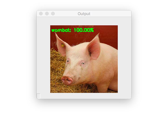
Our input pig.jpg, which was correctly classified as “hog” in the previous section is now labeled as a “wombat”!

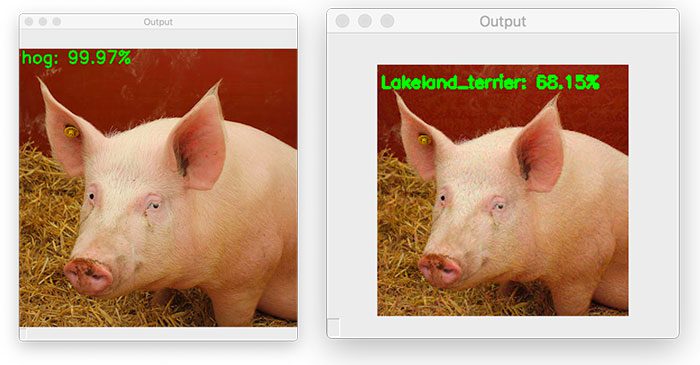
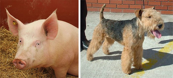
I’ve placed the original pig.jpg image next to the adversarial image generated by our generate_basic_adversary.py script below:

Figure 7: On the left, we have our original input image, which is correctly classified. On the right, we have our output adversarial image, which is incorrectly classified as “wombat” — the human eye is unable to spot any differences between these images.

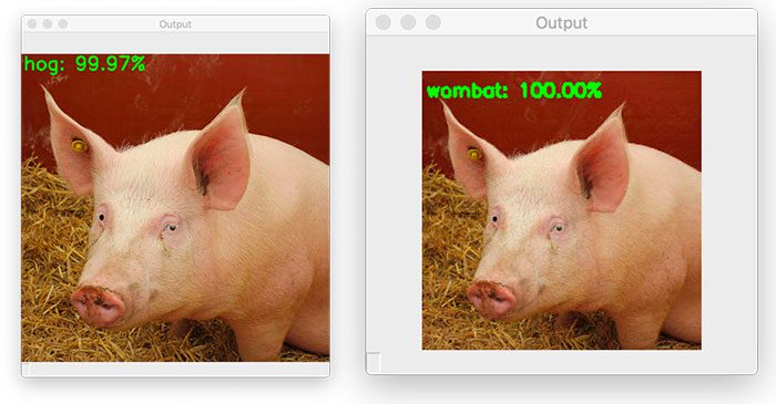
On the left is the original hog image, while on the right we have the output adversarial image, which is incorrectly classified as a “wombat”.

As you can see, there is no perceptible difference between the two images — our human eyes can see the difference between these two images, but to ResNet, they are totally different.

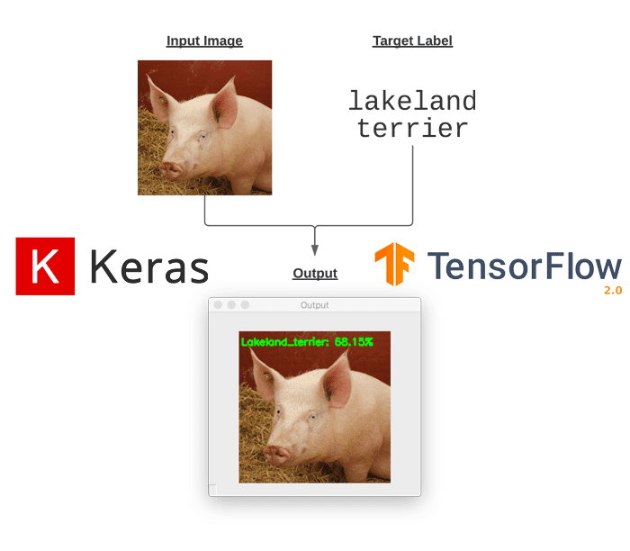
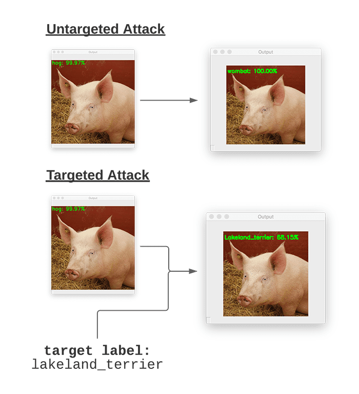
That’s all well and good, but we clearly don’t have control over the final class label in the adversarial image. That raises the question:

Is it possible to control what the final output class label of the input image is? The answer is yes — and I’ll be covering that question in next week’s tutorial.

I’ll conclude by saying that it’s easy to get scared of adversarial images and adversarial attacks if you let your imagination get the best of you. But as we’ll see in a later tutorial on PyImageSearch, we can actually defend against these types of attacks. More on that later.

Credits

This tutorial would not have been possible without the research of Goodfellow, Szegedy, and many other deep learning researchers.

Additionally, I want to call out that the implementation used in today’s tutorial is inspired by TensorFlow’s official implementation of the Fast Gradient Signed Method. I strongly suggest you take a look at their example, which does a fantastic job explaining the more theoretical and mathematically motivated aspects of this tutorial.

What’s next?

Figure 8: If you want to learn to train your own deep learning models on your own datasets, pick up a copy of Deep Learning for Computer Vision with Python, and begin studying! My team and I will be there every step of the way.

Today’s tutorial was the first time we have formally covered both non-adversarial image classification and adversarial images and attacks, with Keras and TensorFlow.

If you don’t already know the fundamentals of deep learning, OR you have begun to envision the creation (and destruction) of your own personal ImageNet dataset – now is the perfect time for you to invest in your education! To get your head start, I personally suggest you read my book Deep Learning for Computer Vision with Python.

I crafted my book so that it perfectly blends theory with code implementation, ensuring you can master:

  • Deep learning fundamentals and theory without unnecessary mathematical fluff. I present the basic equations and back them up with code walkthroughs that you can implement and easily understand. You don’t need a degree in advanced mathematics to understand this book.
  • How to implement your own custom neural network architectures. Not only will you learn how to implement state-of-the-art architectures, including ResNet, SqueezeNet, etc., but you’ll also learn how to create your own custom CNNs.
  • How to train CNNs on your own datasets. Most deep learning tutorials don’t teach you how to work with your own custom datasets. Mine do. You’ll be training CNNs on your own datasets in no time.
  • Object detection (Faster R-CNNs, Single Shot Detectors, and RetinaNet) and instance segmentation (Mask R-CNN). Use these chapters to create your own custom object detectors and segmentation networks.

You’ll also find answers and proven code recipes to:

  • Create and prepare your own custom image datasets for image classification, object detection, and segmentation
  • Work through hands-on tutorials (with lots of code) that not only show you the algorithms behind deep learning for computer vision but their implementations as well
  • Put my tips, suggestions, and best practices into action, ensuring you maximize the accuracy of your models

Beginners and experts alike tend to resonate with my no-nonsense teaching style and high quality content.

If you’re on the fence about taking the next step in your computer vision, deep learning, and artificial intelligence education, be sure to read my Student Success Stories. My readers have gone on to excel in their careers — you can too!

If you’re ready to begin, purchase your copy today. And if you aren’t convinced yet, I’d be happy to send you the full table of contents + sample chapters — simply click here. You can also browse my library of other book and course offerings.

Summary

In this tutorial, you learned about adversarial attacks, how they work, and the threat they pose to a world becoming more and more reliant on Artificial Intelligence and deep neural networks.

We then implemented a basic adversarial attack algorithm using the Keras and TensorFlow deep learning libraries.

Using adversarial attacks, we can purposely perturb an input image such that:

  1. The input image is misclassified
  2. However, to the human eye, the perturbed image looks identical to the original

However, using the method applied here today, we have absolutely no control over what the final class label of the image is — all we’re doing is creating and embedding a noise vector that causes the deep neural network to misclassify the image.

But what if we could control what the final target class label is? For example, is it possible to take an image of a “dog” and construct an adversarial attack such that the Convolutional Neural Network thinks the image is a “cat”?

The answer is yes — and we’ll be covering that exact same topic in next week’s tutorial.

To download the source code to this post (and be notified when future tutorials are published here on PyImageSearch), simply enter your email address in the form below!

Download the Source Code and FREE 17-page Resource Guide

Enter your email address below to get a .zip of the code and a FREE 17-page Resource Guide on Computer Vision, OpenCV, and Deep Learning. Inside you'll find my hand-picked tutorials, books, courses, and libraries to help you master CV and DL!

The post Adversarial images and attacks with Keras and TensorFlow appeared first on PyImageSearch.


Targeted adversarial attacks with Keras and TensorFlow

$
0
0

In this tutorial, you will learn how to perform targeted adversarial attacks and construct targeted adversarial images using Keras, TensorFlow, and Deep Learning.

Last week’s tutorial covered untargeted adversarial learning, which is the process of:

  • Step #1: Accepting an input image and determining its class label using a pre-trained CNN
  • Step #2: Constructing a noise vector that purposely perturbs the resulting image when added to the input image, in such a way that:
    • Step #2a: The input image is incorrectly classified by the pre-trained CNN
    • Step #2b: Yet, to the human eye, the perturbed image is indistinguishable from the original

With untargeted adversarial learning, we don’t care what the new class label of the input image is, provided that it is incorrectly classified by the CNN. For example, the following image shows that we have applied adversarial learning to take an input correctly classified as “hog” and perturbed it such that the image is now incorrectly classified as “wombat”:

Figure 1: On the left, we have our input image, which is correctly classified a “hog”. By constructing an adversarial attack, we can perturb the input image such that it is incorrectly classified (right). However, we have no control over what the final incorrect class label is — can we somehow modify our adversarial attack algorithm such that we have control over the final output label?

In untargeted adversarial learning, we have no control over what the final, perturbed class label is. But what if we wanted to have control? Is that possible?

It is absolutely is — and in order to control the class label of the perturbed image, we need to apply targeted adversarial learning.

The remainder of this tutorial will show you how to apply targeted adversarial learning.

To learn how to perform targeted adversarial learning with Keras and TensorFlow, just keep reading.

Looking for the source code to this post?

Jump Right To The Downloads Section

Targeted adversarial attacks with Keras and TensorFlow

In the first part of this tutorial, we’ll briefly discuss what adversarial attacks and adversarial images are. I’ll then explain the difference between targeted adversarial attacks versus untargeted ones.

Next, we’ll review our project directory structure, and from there, we’ll implement a Python script that will apply targeted adversarial learning using Keras and TensorFlow.

We’ll wrap up this tutorial with a discussion of our results.

What are adversarial attacks? And what are image adversaries?

Figure 2: When performing an adversarial attack, we present an input image (left) to our neural network. We then use gradient descent to construct the noise vector (middle). This noise vector is added to the input image, resulting in a misclassification (right). (Image source: Figure 1 of Explaining and Harnessing Adversarial Examples)

If you are new to adversarial attacks and have not heard of adversarial images before, I suggest you first read my blog post, Adversarial images and attacks with Keras and TensorFlow before reading this guide.

The gist is that adversarial images are purposely constructed to fool pre-trained models.

For example, if a pre-trained CNN is able to correctly classify an input image, an adversarial attack seeks to take that very same image and:

  1. Perturb it such that the image is now incorrectly classified …
  2. … yet the new, perturbed image looks identical to the original (at least to the human eye)

It’s important to understand how adversarial attacks work and how adversarial images are constructed — knowing this will help you train your CNNs such that they can defend against these types of adversarial attacks (a topic that I will cover in a future tutorial).

How is a targeted adversarial attack different from an untargeted one?

Figure 3: When performing an untargeted adversarial attack, we have no control over the output class label. However, when performing a targeted adversarial attack, we are able to incorporate label information into the gradient update process.

Figure 3 above visually shows the difference between an untargeted adversarial attack and a targeted one.

When constructing an untargeted adversarial attack, we have no control over what the final output class label of the perturbed image will be — our only goal is to force the model to incorrectly classify the input image.

Figure 3 (top) is an example of an untargeted adversarial attack. Here, we input the image of a “pig” — the adversarial attack algorithm then perturbs the input image such that it’s misclassified as a “wombat”, but again, we did not specify what the target class label should be (and frankly, the untargeted algorithm doesn’t care, as long as the input image is now incorrectly classified).

On the other hand, targeted adversarial attacks give us more control over what the final predicted label of the perturbed image is.

Figure 3 (bottom) is an example of a targeted adversarial attack. We once again input our image of a “pig”, but we also supply the target class label of the perturbed image (which in this case is a “Lakeland terrier”, a type of dog).

Our targeted adversarial attack algorithm is then able to perturb the input image of the pig such that it is now misclassified as a Lakeland terrier.

You’ll learn how to perform such a targeted adversarial attack in the remainder of this tutorial.

Configuring your development environment

To configure your system for this tutorial, I recommend following either of these tutorials:

Either tutorial will help you configure your system with all the necessary software for this blog post in a convenient Python virtual environment.

That said, are you:

  • Short on time?
  • Learning on your employer’s administratively locked laptop?
  • Wanting to skip the hassle of fighting with package managers, bash/ZSH profiles, and virtual environments?
  • Ready to run the code right now (and experiment with it to your heart’s content)?

Then join PyImageSearch Plus today! Gain access to our PyImageSearch tutorial Jupyter Notebooks, which run on Google’s Colab ecosystem in your browserno installation required.

Project structure

Before we can start implementing targeted adversarial attack with Keras and TensorFlow, we first need to review our project directory structure.

Start by using the “Downloads” section of this tutorial to download the source code and example images. From there, inspect the directory structure:

$ tree --dirsfirst
.
├── pyimagesearch
│   ├── __init__.py
│   ├── imagenet_class_index.json
│   └── utils.py
├── adversarial.png
├── generate_targeted_adversary.py
├── pig.jpg
└── predict_normal.py

1 directory, 7 files

Our directory structure is identical to last week’s guide on Adversarial images and attacks with Keras and TensorFlow.

The pyimagesearch module contains utils.py, a helper utility that loads and parses the ImageNet class label indexes located in imagenet_class_index.json. We covered this helper function in last week’s tutorial and will not be covering the implementation here today — I suggest you read my previous tutorial for more details on it.

We then have two Python scripts:

  1. predict_normal.py: Accepts an input image (pig.jpg), loads our ResNet50 model, and classifies it. The output of this script will be the ImageNet class label index of the predicted class label. This script was also covered in last week’s tutorial, and I will not be reviewing it here. Please refer back to my Adversarial images and attacks with Keras and TensorFlow guide if you would like a review of the implementation.
  2. generate_targeted_adversary.py: Using the output of our predict_normal.py script, we’ll apply a targeted adversarial attack that allows us to perturb the input image such that it is misclassified to a label of our choosing. The output, adversarial.png, will be serialized to disk.

Let’s get to work implementing targeted adversarial attacks!

Step #1: Obtaining original class label predictions using our pre-trained CNN

Before we can perform a targeted adversarial attack, we must first determine what the predicted class label from a pre-trained CNN is.

For the purposes of this tutorial, we’ll be using the ResNet architecture, pre-trained on the ImageNet dataset.

For any given input image, we’ll need to:

  1. Load the image
  2. Preprocess it
  3. Pass it through ResNet
  4. Obtain the class label prediction
  5. Determine the integer index of the class label

Once we have both the integer index of the predicted class label, along with the target class label, we want the network to predict what the image is; then we’ll be able to perform a targeted adversarial attack.

Let’s get started by obtaining the class label prediction and index of the following image of a pig:

Figure 4: Our input image of a “pig”. We’ll be performing a targeted adversarial attack such that this image is incorrectly classified as a “Lakeland terrier” (a type of dog).

To accomplish this task, we’ll be using the predict_normal.py script in our project directory structure. This script was reviewed in last week’s tutorial, so we won’t be reviewing it here today — if you’re interested in seeing the code behind this script, refer to my previous tutorial.

With all that said, start by using the “Downloads” section of this tutorial to download the source code and example images.

$ python predict_normal.py --image pig.jpg
[INFO] loading image...
[INFO] loading pre-trained ResNet50 model...
[INFO] making predictions...
[INFO] hog => 341
[INFO] 1. hog: 99.97%
[INFO] 2. wild_boar: 0.03%
[INFO] 3. piggy_bank: 0.00%
Figure 5: Our pre-trained ResNet model is able to correctly classify this image as “hog”.

Here you can see that our input pig.jpg image is classified as a “hog” with 99.97% confidence.

In our next section, you’ll learn how to perturb this image such that it’s misclassified as a “Lakeland terrier” (a type of dog).

But for now, make note of Line 5 of our terminal output, which shows that the ImageNet class label index of the predicted label “hog” is 341 — we’ll need this value in the next section.

Step #2: Implementing targeted adversarial attacks with Keras and TensorFlow

We are now ready to implement targeted adversarial attacks and construct a targeted adversarial image using Keras and TensorFlow.

Open up the generate_targeted_adversary.py file in your project directory structure, and insert the following code:

# import necessary packages
from tensorflow.keras.optimizers import Adam
from tensorflow.keras.applications import ResNet50
from tensorflow.keras.losses import SparseCategoricalCrossentropy
from tensorflow.keras.applications.resnet50 import decode_predictions
from tensorflow.keras.applications.resnet50 import preprocess_input
import tensorflow as tf
import numpy as np
import argparse
import cv2

We start by importing our required Python packages on Lines 2-10. Our tf.keras imports include the:

  • Adam optimizer
  • ResNet50 architecture
  • SparseCategoricalCrossentropy loss function
  • ImageNet label decoder function, decode_predictions
  • Image preprocessing utility, preprocess_input

With our imports defined, let’s create a function used to preprocess our input image:

def preprocess_image(image):
	# swap color channels, resize the input image, and add a batch
	# dimension
	image = cv2.cvtColor(image, cv2.COLOR_BGR2RGB)
	image = cv2.resize(image, (224, 224))
	image = np.expand_dims(image, axis=0)

	# return the preprocessed image
	return image

The preprocess_image method accepts a single required argument, the image, which we wish to preprocess. Our image is preprocessed by swapping channel ordering from BGR to RGB, calling preprocess_input to scale the pixel intensities, resizing the image to 224×224 pixels, and adding a batch dimension.

The preprocessed image is then returned to the calling function.

Our next function, clip_eps, clips values of the input tensor to the range [-eps, eps]:

def clip_eps(tensor, eps):
	# clip the values of the tensor to a given range and return it
	return tf.clip_by_value(tensor, clip_value_min=-eps,
		clip_value_max=eps)

We accomplish this clipping by using TensorFlow’s clip_by_value method. We supply the tensor as an input, and then set -eps as the minimum clip value limit, along with eps as the positive clip value limit.

This function will be used when we construct our perturbation vector, ensuring that the noise vector we construct falls within tolerable limits, and most importantly, does not significantly impact the visual quality of the output adversarial image.

Keep in mind that adversarial images should be identical (to the human eye) to their original inputs — by clipping tensor values within tolerable limits, we are able to enforce this requirement.

Next, we need to define the generate_targeted_adversaries function, which is the workhorse of this Python script:

def generate_targeted_adversaries(model, baseImage, delta, classIdx,
	target, steps=500):
	# iterate over the number of steps
	for step in range(0, steps):
		# record our gradients
		with tf.GradientTape() as tape:
			# explicitly indicate that our perturbation vector should
			# be tracked for gradient updates
			tape.watch(delta)

			# add our perturbation vector to the base image and
			# preprocess the resulting image
			adversary = preprocess_input(baseImage + delta)

Our generated_targeted_adversaries function accepts five parameters, including a fifth optional one:

  • model: Our ResNet50 model (you could swap in a different pre-trained model such as VGG16, MobileNet, etc. if you prefer).
  • baseImage: The original non-perturbed input image that we wish to construct an adversarial attack for, causing our model to misclassify it.
  • delta: Our noise vector, which will be added to the baseImage , ultimately causing the misclassification. We’ll update this delta vector by means of gradient descent.
  • classIdx: The integer class label index we obtained by running the predict_normal.py script.
  • steps: Number of gradient descent steps to perform (defaults to 50 steps).

Line 30 starts a loop over the number of steps of gradient descent we are going to apply. For each step, we will record our gradients (Line 32), and specifically, watch the delta variable (Line 35). The delta value is the perturbation vector we are generating.

Line 39 creates our image adversary by adding the delta perturbation vector to the baseImage (i.e., original input image), the result of which is our adversary image. We then preprocess the generated adversary.

Next comes the gradient descent portion of applying a targeted adversarial attack:

			# run this newly constructed image tensor through our
			# model and calculate the loss with respect to the
			# both the *original* class label and the *target*
			# class label
			predictions = model(adversary, training=False)
			originalLoss = -sccLoss(tf.convert_to_tensor([classIdx]),
				predictions)
			targetLoss = sccLoss(tf.convert_to_tensor([target]),
				predictions)
			totalLoss = originalLoss + targetLoss

			# check to see if we are logging the loss value, and if
			# so, display it to our terminal
			if step % 20 == 0:
				print("step: {}, loss: {}...".format(step,
					totalLoss.numpy()))

		# calculate the gradients of loss with respect to the
		# perturbation vector
		gradients = tape.gradient(totalLoss, delta)

		# update the weights, clip the perturbation vector, and
		# update its value
		optimizer.apply_gradients([(gradients, delta)])
		delta.assign_add(clip_eps(delta, eps=EPS))

	# return the perturbation vector
	return delta

Line 45 makes predictions on the adversary image (i.e., probability predictions for each class label in the ImageNet dataset).

We then compute three loss outputs on Lines 46-50:

  1. originalLoss: Computes the negative sparse categorical cross-entropy loss with respect to the original class label.
  2. targetLoss: Derives the positive categorical cross-entropy loss with respect to the target class label (i.e., what we want the image adversary to be misclassified as, hence the term targeted adversarial attack). We take the negative/positive signs that way because our objective is to minimize the probability for the true class and maximize the probability of the target class.
  3. totalLoss: Sum of the original loss and the targeted loss.

Every 20 steps, we display the loss to our terminal (Lines 54-56).

Outside of the with statement now, we calculate the gradients of the loss with respect to our perturbation vector (Line 55).

Given the gradients, we apply them to our delta, and then clip values inside delta to our epsilon (EPS) limits.

Again, keep in mind that the clip_eps function is used to ensure that the noise vector we construct falls within tolerable limits, and most importantly, does not significantly impact the visual quality of the output adversarial image.

Finally, we return the resulting perturbation vector to the calling function — the final delta value will allow us to construct the adversarial attack used to fool our model.

With all of our functions now defined, we can move to parsing command line arguments:

# construct the argument parser and parse the arguments
ap = argparse.ArgumentParser()
ap.add_argument("-i", "--input", required=True,
	help="path to original input image")
ap.add_argument("-o", "--output", required=True,
	help="path to output adversarial image")
ap.add_argument("-c", "--class-idx", type=int, required=True,
	help="ImageNet class ID of the predicted label")
ap.add_argument("-t", "--target-class-idx", type=int, required=True,
	help="ImageNet class ID of the target adversarial label")
args = vars(ap.parse_args())

Our generate_targeted_adversary.py script requires four command line arguments:

  • --input: The path to our input image.
  • --output: The path to our output adversarial image after the targeted adversarial attack has been performed.
  • --class-idx: The integer class label index from the ImageNet dataset. We obtained this value by running predict_normal.py in the “Non-adversarial image classification results” section of the prior tutorial.
  • --target-class-idx: The ImageNet class label index of what we want the input image to be incorrectly classified as (you’ll see an example of how to select this class label integer value in the “Step #3: Targeted adversarial attack results” section below).

Let’s move on to a few initializations:

EPS = 2 / 255.0
LR = 5e-3

# load image from disk and preprocess it
print("[INFO] loading image...")
image = cv2.imread(args["input"])
image = preprocess_image(image)

Line 82 defines our epsilon (EPS) value used for clipping tensors when constructing the adversarial image. An EPS value of 2 / 255.0 is a standard value used in adversarial publications and tutorials.

We then define our learning rate on Line 84. A value of LR = 5e-3 was obtained by empirical tuning — you may need to update this value when constructing your own targeted adversarial attacks.

Lines 88 and 89 load our input image and then preprocess it using ResNet’s preprocessing helper function.

Next, we need to load the ResNet model and initialize our loss function:

# load the pre-trained ResNet50 model for running inference
print("[INFO] loading pre-trained ResNet50 model...")
model = ResNet50(weights="imagenet")

# initialize optimizer and loss function
optimizer = Adam(learning_rate=LR)
sccLoss = SparseCategoricalCrossentropy()

# create a tensor based off the input image and initialize the
# perturbation vector (we will update this vector via training)
baseImage = tf.constant(image, dtype=tf.float32)
delta = tf.Variable(tf.zeros_like(baseImage), trainable=True)

In this code block we:

  • Load ResNet50 from disk with weights pre-trained on the ImageNet dataset
  • Indicate that the Adam optimizer will be used when applying gradient descent
  • Initialize our sparse categorical cross-entropy loss function
  • Convert our input image to a TensorFlow constant (since the input image will not be updated during gradient descent)
  • Construct a variable for our delta (i.e., the perturbation vector) with the same spatial dimensions as the input image

If you would like more details on these variables and initializations, refer to last week’s tutorial where I cover them in more detail.

With all of our variables constructed, we can now apply the targeted adversarial attack:

# generate the perturbation vector to create an adversarial example
print("[INFO] generating perturbation...")
deltaUpdated = generate_targeted_adversaries(model, baseImage, delta,
	args["class_idx"], args["target_class_idx"])

# create the adversarial example, swap color channels, and save the
# output image to disk
print("[INFO] creating targeted adversarial example...")
adverImage = (baseImage + deltaUpdated).numpy().squeeze()
adverImage = np.clip(adverImage, 0, 255).astype("uint8")
adverImage = cv2.cvtColor(adverImage, cv2.COLOR_RGB2BGR)
cv2.imwrite(args["output"], adverImage)

A call to generate_targeted_adversaries generates our final deltaUpdated value, which is the perturbation vector used to construct the targeted adversarial attack.

From there, we construct adverImage, our final adversarial image, by adding the perturbation vector to the original input image.

We then clip any pixel values such that all pixels are in the range [0, 255], followed by converting the image to an unsigned 8-bit integer (such that OpenCV can operate on the image).

The final adverImage is then written to disk.

The question remains — have we fooled our original ResNet model into making an incorrect prediction?

Let’s answer that question in the following code block:

# run inference with this adversarial example, parse the results,
# and display the top-1 predicted result
print("[INFO] running inference on the adversarial example...")
preprocessedImage = preprocess_input(baseImage + deltaUpdated)
predictions = model.predict(preprocessedImage)
predictions = decode_predictions(predictions, top=3)[0]
label = predictions[0][1]
confidence = predictions[0][2] * 100
print("[INFO] label: {} confidence: {:.2f}%".format(label,
	confidence))

# write the top-most predicted label on the image along with the
# confidence score
text = "{}: {:.2f}%".format(label, confidence)
cv2.putText(adverImage, text, (3, 20), cv2.FONT_HERSHEY_SIMPLEX, 0.5,
	(0, 255, 0), 2)

# show the output image
cv2.imshow("Output", adverImage)
cv2.waitKey(0)

Line 120 constructs a preprocessedImage by first constructing the adversarial image and then preprocessing it using ResNet’s preprocessing utility.

Once the image is preprocessed, we make predictions on it using our model. These predictions are then decoded and the top #1 prediction obtained — the class label and corresponding probability are then displayed to our terminal (Lines 121-126).

Finally, we annotate our output image with the predicted label and confidence, and then display the output image to our screen.

That was quite a lot of code to review! Take a second to congratulate yourself on a successful implementation of targeted adversarial attacks. In the next section, we’ll see the fruits of our hard work.

Step #3: Targeted adversarial attack results

We are now ready to perform a targeted adversarial attack! Make sure you’ve used the “Downloads” section of this tutorial to download the source code and example images.

Next, open up the imagenet_class_index.json file and determine the integer index of the ImageNet class label we want to “fool” the network into predicting — the first few lines of the class label index file look like this:

{
  "0": [
    "n01440764",
    "tench"
  ],
  "1": [
    "n01443537",
    "goldfish"
  ],
  "2": [
    "n01484850",
    "great_white_shark"
  ],
  "3": [
    "n01491361",
    "tiger_shark"
  ],
...

Scroll through the file until you find a class label you want to use.

In this case, I have chosen index 189, which corresponds to a “Lakeland terrier” (a type of dog):

...
"189": [
    "n02095570",
    "Lakeland_terrier"
  ],
...

From there, you can open up a terminal and execute the following command:

$ python generate_targeted_adversary.py --input pig.jpg --output adversarial.png --class-idx 341 --target-class-idx 189
[INFO] loading image...
[INFO] loading pre-trained ResNet50 model...
[INFO] generating perturbation...
step: 0, loss: 16.111093521118164...
step: 20, loss: 15.760734558105469...
step: 40, loss: 10.959839820861816...
step: 60, loss: 7.728139877319336...
step: 80, loss: 5.327273368835449...
step: 100, loss: 3.629972219467163...
step: 120, loss: 2.3259339332580566...
step: 140, loss: 1.259613037109375...
step: 160, loss: 0.30303144454956055...
step: 180, loss: -0.48499584197998047...
step: 200, loss: -1.158257007598877...
step: 220, loss: -1.759873867034912...
step: 240, loss: -2.321563720703125...
step: 260, loss: -2.910153865814209...
step: 280, loss: -3.470625877380371...
step: 300, loss: -4.021825313568115...
step: 320, loss: -4.589465141296387...
step: 340, loss: -5.136003017425537...
step: 360, loss: -5.707150459289551...
step: 380, loss: -6.300693511962891...
step: 400, loss: -7.014866828918457...
step: 420, loss: -7.820181369781494...
step: 440, loss: -8.733556747436523...
step: 460, loss: -9.780607223510742...
step: 480, loss: -10.977422714233398...
[INFO] creating targeted adversarial example...
[INFO] running inference on the adversarial example...
[INFO] label: Lakeland_terrier confidence: 54.82%
Figure 6: Our original input was correctly classified as “hog” (left); however, our targeted adversarial attack now results in the image being incorrectly classified as a “Lakeland terrier” (right).

On the left, you can see our original input image, which was correctly classified as “hog”.

We then applied a targeted adversarial attack (right) that perturbed the input image such that it has been misclassified as a Lakeland terrier (a type of dog) with 68.15% confidence!

For reference, a Lakeland terrier looks nothing like a pig:

Figure 7: A “Lakeland terrier” (right) looks nothing like a “hog” (left), thus demonstrating the power of targeted adversarial attacks.

In last week’s tutorial on untargeted adversarial attacks, we saw that we have no control over the final predicted class label of the perturbed image; however, by applying a targeted adversarial attack, we are able to control what label is ultimately predicted.

What’s next?

Figure 8: My Deep Learning for Computer Vision with Python course is the go-to resource for deep learning hobbyists, practitioners, and experts. Use this book to build your skillset from the bottom up, or read it to gain a deeper understanding of AI. My team and I will be there every step of the way.

Great work keeping up with my ‘Adversarial Images’ series! Successfully completing the implementation of targeted adversarial learning to control predicted class labels of perturbed images is tough stuff!

In the domain of adversarial machine learning, attacking and defending is of ultimate importance when creating and training your own model.

To get up to speed on all deep learning applications in the AI industry, I suggest you read my book Deep Learning for Computer Vision with Python.

I crafted this book so it perfectly blends theory with code implementation, ensuring you can master:

  • Deep learning fundamentals and theory without unnecessary mathematical fluff. I present the basic equations and back them up with code walkthroughs that you can implement and easily understand. You don’t need a degree in advanced mathematics to understand this book.
  • How to implement your own custom neural network architectures. Not only will you learn how to implement state-of-the-art architectures, including ResNet, SqueezeNet, etc., but you’ll also learn how to create your own custom CNNs.
  • How to train CNNs on your own datasets. Most deep learning tutorials don’t teach you how to work with your own custom datasets. Mine do. You’ll be training CNNs on your own datasets in no time.
  • Object detection (Faster R-CNNs, Single Shot Detectors, and RetinaNet) and instance segmentation (Mask R-CNN). Use these chapters to create your own custom object detectors and segmentation networks.

You’ll also find answers and proven code recipes to:

  • Create and prepare your own custom image datasets for image classification, object detection, and segmentation
  • Work through hands-on tutorials (with lots of code) that not only show you the algorithms behind deep learning for computer vision but their implementations as well
  • Put my tips, suggestions, and best practices into action, ensuring you maximize the accuracy of your models

Beginners and experts alike tend to resonate with my no-nonsense teaching style and high quality content.

If you’re ready to begin a course at your own pace, purchase your copy today. And if you aren’t convinced yet, I’d be happy to send you the full table of contents + sample chapters — simply click here. You can also browse my library of other book and course offerings.

Summary

In this tutorial, you learned how to perform targeted adversarial learning using Keras, TensorFlow, and Deep Learning.

When applying untargeted adversarial learning, our goal is to perturb an input image such that:

  1. The perturbed image is misclassified by our pre-trained CNN
  2. Yet, to the human eye, the perturbed image is identical to the original

The problem with untargeted adversarial learning is that we have no control over the perturbed output class label. For example, if we have an input image of a “pig”, and we want to perturb that image such that it’s misclassified, we cannot control what the new class label will be.

Targeted adversarial learning on the other hand allows us to control what the new class label will be — and it’s super easy to implement, requiring only an update to our loss function computation.

So far, we have covered how to construct adversarial attacks, but what if we wanted to defend against them. Is that possible?

It certainly is — I’ll cover defending against adversarial attacks in a future blog post.

To download the source code to this post (and be notified when future tutorials are published here on PyImageSearch), simply enter your email address in the form below!

Download the Source Code and FREE 17-page Resource Guide

Enter your email address below to get a .zip of the code and a FREE 17-page Resource Guide on Computer Vision, OpenCV, and Deep Learning. Inside you'll find my hand-picked tutorials, books, courses, and libraries to help you master CV and DL!

The post Targeted adversarial attacks with Keras and TensorFlow appeared first on PyImageSearch.

OpenCV Super Resolution with Deep Learning

$
0
0

In this tutorial you will learn how to perform super resolution in images and real-time video streams using OpenCV and Deep Learning.

Today’s blog post is inspired by an email I received from PyImageSearch reader, Hisham:

“Hi Adrian, I read your Deep Learning for Computer Vision with Python book and went through your super resolution implementation with Keras and TensorFlow. It was super helpful, thank you.

I was wondering:

Are there any pre-trained super resolution models compatible with OpenCV’s dnn module?

Can they work in real-time?

If you have any suggestions, that would be a big help.”

You’re in luck, Hisham — there are super resolution deep neural networks that are both:

  1. Pre-trained (meaning you don’t have to train them yourself on a dataset)
  2. Compatible with OpenCV

However, OpenCV’s super resolution functionality is actually “hidden” in a submodule named in dnn_superres in an obscure function called DnnSuperResImpl_create.

The function requires a bit of explanation to use, so I decided to author a tutorial on it; that way everyone can learn how to use OpenCV’s super resolution functionality.

By the end of this tutorial, you’ll be able to perform super resolution with OpenCV in both images and real-time video streams!

To learn how to use OpenCV for deep learning-based super resolution, just keep reading.

Looking for the source code to this post?

Jump Right To The Downloads Section

OpenCV Super Resolution with Deep Learning

In the first part of this tutorial, we will discuss:

  • What super resolution is
  • Why we can’t use simple nearest neighbor, linear, or bicubic interpolation to substantially increase the resolution of images
  • How specialized deep learning architectures can help us achieve super resolution in real-time

From there, I’ll show you how to implement OpenCV super resolution with both:

  1. Images
  2. Real-time video resolutions

We’ll wrap up this tutorial with a discussion of our results.

What is super resolution?

Super resolution encompases a set of algorithms and techniques used to enhance, increase, and upsample the resolution of an input image. More simply, take an input image and increase the width and height of the image with minimal (and ideally zero) degradation in quality.

That’s a lot easier said than done.

Anyone who has ever opened a small image in Photoshop or GIMP and then tried to resize it knows that the output image ends up looking pixelated.

That’s because Photoshop, GIMP, Image Magick, OpenCV (via the cv2.resize function), etc. all use classic interpolation techniques and algorithms (ex., nearest neighbor interpolation, linear interpolation, bicubic interpolation) to increase the image resolution.

These functions “work” in the sense that an input image is presented, the image is resized, and then the resized image is returned to the calling function …

… however, if you increase the spatial dimensions too much, then the output image appears pixelated, has artifacts, and in general, just looks “aesthetically unpleasing” to the human eye.

For example, let’s consider the following figure:

Figure 1: On the top we have our original input image. We wish to increase the resolution of the area in the red rectangle. Applying bicubic interpolation to this region yields poor results.

On the top we have our original image. The area highlighted in the red rectangle is the area we wish to extract and increase the resolution of (i.e., resize to a larger width and height without degrading the quality of the image patch).

On the bottom we have the output of applying bicubic interpolation, the standard interpolation method used for increasing the size of input images (and what we commonly use in cv2.resize when needing to increase the spatial dimensions of an input image).

However, take a second to note how pixelated, blurry, and just unreadable the image patch is after applying bicubic interpolation.

That raises the question:

Is there a better way to increase the resolution of the image without degrading the quality?

The answer is yes — and it’s not magic either. By applying novel deep learning architectures, we’re able to generate high resolution images without these artifacts:

Figure 2: On the top we have our original input image. The middle shows the output of applying bicubic interpolation to the area in the red rectangle. Finally, the bottom displays the output of a super resolution deep learning model. The resulting image is significantly more clear.

Again, on the top we have our original input image. In the middle we have low quality resizing after applying bicubic interpolation. And on the bottom we have the output of applying our super resolution deep learning model.

The difference is like night and day. The output deep neural network super resolution model is crisp, easy to read, and shows minimal signs of resizing artifacts.

In the rest of this tutorial, I’ll uncover this “magic” and show you how to perform super resolution with OpenCV!

OpenCV super resolution models

Figure 3: Example of a super resolution architecture compatible with the OpenCV library (image source).

We’ll be utilizing four pre-trained super resolution models in this tutorial. A review of the model architectures, how they work, and the training process of each respective model is outside the scope of this guide (as we’re focusing on implementation only).

If you would like to read more about these models, I’ve included their names, implementations, and paper links below:

A big thank you to Taha Anwar from BleedAI for putting together his guide on OpenCV super resolution, which curated much of this information — it was immensely helpful when authoring this piece.

Configuring your development environment for super resolution with OpenCV

In order to apply OpenCV super resolution, you must have OpenCV 4.3 (or greater) installed on your system. While the dnn_superes module was implemented in C++ back in OpenCV 4.1.2, the Python bindings were not implemented until OpenCV 4.3.

Luckily, OpenCV 4.3+ is pip-installable:

$ pip install opencv-contrib-python

If you need help configuring your development environment for OpenCV 4.3+, I highly recommend that you read my pip install OpenCV guide — it will have you up and running in a matter of minutes.

Having problems configuring your development environment?

Figure 4: Having trouble configuring your dev environment? Want access to pre-configured Jupyter Notebooks running on Google Colab? Be sure to join PyImageSearch Plus — you’ll be up and running with this tutorial in a matter of minutes.

All that said, are you:

  • Short on time?
  • Learning on your employer’s administratively locked system?
  • Wanting to skip the hassle of fighting with the command line, package managers, and virtual environments?
  • Ready to run the code right now on your Windows, macOS, or Linux system?

Then join PyImageSearch Plus today!

Gain access to Jupyter Notebooks for this tutorial and other PyImageSearch guides that are pre-configured to run on Google Colab’s ecosystem right in your web browser! No installation required.

And best of all, these Jupyter Notebooks will run on Windows, macOS, and Linux!

Project structure

With our development environment configured, let’s move on to reviewing our project directory structure:

$ tree . --dirsfirst
.
├── examples
│   ├── adrian.png
│   ├── butterfly.png
│   ├── jurassic_park.png
│   └── zebra.png
├── models
│   ├── EDSR_x4.pb
│   ├── ESPCN_x4.pb
│   ├── FSRCNN_x3.pb
│   └── LapSRN_x8.pb
├── super_res_image.py
└── super_res_video.py

2 directories, 10 files

Here you can see that we have two Python scripts to review today:

  1. super_res_image.py: Performs OpenCV super resolution in images loaded from disk
  2. super_res_video.py: Applies super resolution with OpenCV to real-time video streams

We’ll be covering the implementation of both Python scripts in detail later in this post.

From there, we have four super resolution models:

  1. EDSR_x4.pb: Model from the Enhanced Deep Residual Networks for Single Image Super-Resolution paper — increases the input image resolution by 4x
  2. ESPCN_x4.pb: Super resolution model from Real-Time Single Image and Video Super-Resolution Using an Efficient Sub-Pixel Convolutional Neural Networkincreases resolution by 4x
  3. FSRCNN_x3.pb: Model from Accelerating the Super-Resolution Convolutional Neural Networkincreases image resolution by 3x
  4. LapSRN_x8.pb: Super resolution model from Fast and Accurate Image Super-Resolution with Deep Laplacian Pyramid Networksincreases image resolution by 8x

Finally, the examples directory contains example input images that we’ll be applying OpenCV super resolution to.

Implementing OpenCV super resolution with images

We are now ready to implement OpenCV super resolution in images!

Open up the super_res_image.py file in your project directory structure, and let’s get to work:

# import the necessary packages
import argparse
import time
import cv2
import os

# construct the argument parser and parse the arguments
ap = argparse.ArgumentParser()
ap.add_argument("-m", "--model", required=True,
	help="path to super resolution model")
ap.add_argument("-i", "--image", required=True,
	help="path to input image we want to increase resolution of")
args = vars(ap.parse_args())

Lines 2-5 import our required Python packages. We’ll use the dnn_superres submodule of cv2 (our OpenCV bindings) to perform super resolution later in this script.

From there, Lines 8-13 parse our command line arguments. We only need two command line arguments here:

  1. --model: The path to the input OpenCV super resolution model
  2. --image: The path to the input image that we want to apply super resolution to

Given our super resolution model path, we now need to extract the model name and the model scale (i.e., factor by which we’ll be increasing the image resolution):

# extract the model name and model scale from the file path
modelName = args["model"].split(os.path.sep)[-1].split("_")[0].lower()
modelScale = args["model"].split("_x")[-1]
modelScale = int(modelScale[:modelScale.find(".")])

Line 16 extracts the modelName, which can be EDSR, ESPCN, FSRCNN, or LapSRN, respectively. The modelNamehas to be one of these model names; otherwise, the dnn_superres module and DnnSuperResImpl_create function will not work.

We then extract the modelScale from the input --model path (Lines 17 and 18).

Both the modelName and modelPath are displayed to our terminal (just in case we need to perform any debugging).

With the model name and scale parsed, we can now move on to loading the OpenCV super resolution model:

# initialize OpenCV's super resolution DNN object, load the super
# resolution model from disk, and set the model name and scale
print("[INFO] loading super resolution model: {}".format(
	args["model"]))
print("[INFO] model name: {}".format(modelName))
print("[INFO] model scale: {}".format(modelScale))
sr = cv2.dnn_superres.DnnSuperResImpl_create()
sr.readModel(args["model"])
sr.setModel(modelName, modelScale)

We start by instantiating an instance of DnnSuperResImpl_create, which is our actual super resolution object.

A call to readModel loads our OpenCV super resolution model from disk.

We then have to make a call to setModel to explicitly set the modelName and modelScale.

Failing to either read the model from disk or set the model name and scale will result in our super resolution script either erroring out or segfaulting.

Let’s now perform super resolution with OpenCV:

# load the input image from disk and display its spatial dimensions
image = cv2.imread(args["image"])
print("[INFO] w: {}, h: {}".format(image.shape[1], image.shape[0]))

# use the super resolution model to upscale the image, timing how
# long it takes
start = time.time()
upscaled = sr.upsample(image)
end = time.time()
print("[INFO] super resolution took {:.6f} seconds".format(
	end - start))

# show the spatial dimensions of the super resolution image
print("[INFO] w: {}, h: {}".format(upscaled.shape[1],
	upscaled.shape[0]))

Lines 31 and 32 load our input --image from disk and display the original width and height.

From there, Line 37 makes a call to sr.upsample, supplying the original input image. The upsample function, as the name suggests, performs a forward pass of our OpenCV super resolution model, returning the upscaled image.

We take care to measure the wall time for how long the super resolution process takes, followed by displaying the new width and height of our upscaled image to our terminal.

For comparison, let’s apply standard bicubic interpolation and time how long it takes:

# resize the image using standard bicubic interpolation
start = time.time()
bicubic = cv2.resize(image, (upscaled.shape[1], upscaled.shape[0]),
	interpolation=cv2.INTER_CUBIC)
end = time.time()
print("[INFO] bicubic interpolation took {:.6f} seconds".format(
	end - start))

Bicubic interpolation is the standard algorithm used to increase the resolution of an image. This method is implemented in nearly every image processing tool and library, including Photoshop, GIMP, Image Magick, PIL/PIllow, OpenCV, Microsoft Word, Google Docs, etc. — if a piece of software needs to manipulate images, it more than likely implements bicubic interpolation.

Finally, let’s display the output results to our screen:

# show the original input image, bicubic interpolation image, and
# super resolution deep learning output
cv2.imshow("Original", image)
cv2.imshow("Bicubic", bicubic)
cv2.imshow("Super Resolution", upscaled)
cv2.waitKey(0)

Here we display our original input image, the bicubic resized image, and finally our upscaled super resolution image.

We display the three results to our screen so we can easily compare results.

OpenCV super resolution results

Start by making sure you’ve used the “Downloads” section of this tutorial to download the source code, example images, and pre-trained super resolution models.

From there, open up a terminal, and execute the following command:

$ python super_res_image.py --model models/EDSR_x4.pb --image examples/adrian.png
[INFO] loading super resolution model: models/EDSR_x4.pb
[INFO] model name: edsr
[INFO] model scale: 4
[INFO] w: 100, h: 100
[INFO] super resolution took 1.183802 seconds
[INFO] w: 400, h: 400
[INFO] bicubic interpolation took 0.000565 seconds
Figure 5: Applying the EDSR model for super resolution with OpenCV.

In the top we have our original input image. In the middle we have applied the standard bicubic interpolation image to increase the dimensions of the image. Finally, the bottom shows the output of the EDSR super resolution model (increasing the image dimensions by 4x).

If you study the two images, you’ll see that the super resolution images appear “more smooth.” In particular, take a look at my forehead region. In the bicubic image, there is a lot of pixelation going on — but in the super resolution image, my forehead is significantly more smooth and less pixelated.

The downside to the EDSR super resolution model is that it’s a bit slow. Standard bicubic interpolation could take a 100x100px image and increase it to 400x400px at the rate of > 1700 frames per second.

EDSR, on the other hand, takes greater than one second to perform the same upsampling. Therefore, EDSR is not suitable for real-time super resolution (at least not without a GPU).

Note: All timings here were collected with a 3 GHz Intel Xeon W processor. A GPU was not used.

Let’s try another image, this one of a butterfly:

$ python super_res_image.py --model models/ESPCN_x4.pb --image examples/butterfly.png
[INFO] loading super resolution model: models/ESPCN_x4.pb
[INFO] model name: espcn
[INFO] model scale: 4
[INFO] w: 400, h: 240
[INFO] super resolution took 0.073628 seconds
[INFO] w: 1600, h: 960
[INFO] bicubic interpolation took 0.000833 seconds
Figure 6: The result of applying the ESPCN for super resolution with OpenCV.

Again, on the top we have our original input image. After applying standard bicubic interpolation we have the middle image. And on the bottom we have the output of applying the ESPCN super resolution model.

The best way you can see the difference between these two super resolution models is to study the butterfly’s wings. Notice how the bicubic interpolation method looks more noisy and distorted, while the ESPCN output image is significantly more smooth.

The good news here is that the ESPCN model is significantly faster, capable of taking a 400x240px image and upsampling it to a 1600x960px model at the rate of 13 FPS on a CPU.

The next example applies the FSRCNN super resolution model:

$ python super_res_image.py --model models/FSRCNN_x3.pb --image examples/jurassic_park.png
[INFO] loading super resolution model: models/FSRCNN_x3.pb
[INFO] model name: fsrcnn
[INFO] model scale: 3
[INFO] w: 350, h: 197
[INFO] super resolution took 0.082049 seconds
[INFO] w: 1050, h: 591
[INFO] bicubic interpolation took 0.001485 seconds
Figure 7: Applying the FSRCNN model for OpenCV super resolution.

Pause a second and take a look at Allen Grant’s jacket (the man wearing the blue denim shirt). In the bicubic interpolation image, this shirt is grainy. But in the FSRCNN output, the jacket is far more smoothed.

Similar to the ESPCN super resolution model, FSRCNN took only 0.08 seconds to upsample the image (a rate of ~12 FPS).

Finally, let’s look at the LapSRN model, which will increase our input image resolution by 8x:

$ python super_res_image.py --model models/LapSRN_x8.pb --image examples/zebra.png
[INFO] loading super resolution model: models/LapSRN_x8.pb
[INFO] model name: lapsrn
[INFO] model scale: 8
[INFO] w: 400, h: 267
[INFO] super resolution took 4.759974 seconds
[INFO] w: 3200, h: 2136
[INFO] bicubic interpolation took 0.008516 seconds
Figure 8: Using the LapSRN model to increase the image resolution by 8x with OpenCV super resolution.

Perhaps unsurprisingly, this model is the slowest, taking over 4.5 seconds to increase the resolution of a 400x267px input to an output of 3200x2136px. Given that we are increasing the spatial resolution by 8x, this timing result makes sense.

That said, the output of the LapSRN super resolution model is fantastic. Look at the zebra stripes between the bicubic interpolation output (middle) and the LapSRN output (bottom). The stripes on the zebra are crisp and defined, unlike the bicubic output.

Implementing real-time super resolution with OpenCV

We’ve seen super resolution applied to single images — but what about real-time video streams?

Is it possible to perform OpenCV super resolution in real-time?

The answer is yes, it’s absolutely possible — and that’s exactly what our super_res_video.py script does.

Note: Much of the super_res_video.py script is similar to our super_res_image.py script, so I will spend less time explaining the real-time implementation. Refer back to the previous section on “Implementing OpenCV super resolution with images” if you need additional help understanding the code.

Let’s get started:

# import the necessary packages
from imutils.video import VideoStream
import argparse
import imutils
import time
import cv2
import os

# construct the argument parser and parse the arguments
ap = argparse.ArgumentParser()
ap.add_argument("-m", "--model", required=True,
	help="path to super resolution model")
args = vars(ap.parse_args())

Lines 2-7 import our required Python packages. These are all near-identical to our previous script on super resolution with images, with the exception of my imutils library and the VideoStream implementation from it.

We then parse our command line arguments. Only a single argument is required, --model, which is the path to our input super resolution model.

Next, let’s extract the model name and model scale, followed by loading our OpenCV super resolution model from disk:

# extract the model name and model scale from the file path
modelName = args["model"].split(os.path.sep)[-1].split("_")[0].lower()
modelScale = args["model"].split("_x")[-1]
modelScale = int(modelScale[:modelScale.find(".")])

# initialize OpenCV's super resolution DNN object, load the super
# resolution model from disk, and set the model name and scale
print("[INFO] loading super resolution model: {}".format(
	args["model"]))
print("[INFO] model name: {}".format(modelName))
print("[INFO] model scale: {}".format(modelScale))
sr = cv2.dnn_superres.DnnSuperResImpl_create()
sr.readModel(args["model"])
sr.setModel(modelName, modelScale)

# initialize the video stream and allow the camera sensor to warm up
print("[INFO] starting video stream...")
vs = VideoStream(src=0).start()
time.sleep(2.0)

Lines 16-18 extract our modelName and modelScale from the input --model file path.

Using that information, we instantiate our super resolution (sr) object, load the model from disk, and set the model name and scale (Lines 26-28).

We then initialize our VideoStream (such that we can read frames from our webcam) and allow the camera sensor to warm up.

With our initializations taken care of, we can now loop over frames from the VideoStream:

# loop over the frames from the video stream
while True:
	# grab the frame from the threaded video stream and resize it
	# to have a maximum width of 300 pixels
	frame = vs.read()
	frame = imutils.resize(frame, width=300)

	# upscale the frame using the super resolution model and then
	# bicubic interpolation (so we can visually compare the two)
	upscaled = sr.upsample(frame)
	bicubic = cv2.resize(frame,
		(upscaled.shape[1], upscaled.shape[0]),
		interpolation=cv2.INTER_CUBIC)

Line 36 starts looping over frames from our video stream. We then grab the next frame and resize it to have a width of 300px.

We perform this resizing operation for visualization/example purposes. Recall that the point of this tutorial is to apply super resolution with OpenCV. Therefore, our example should show how to take a low resolution input and then generate a high resolution output (which is exactly why we are reducing the resolution of the frame).

Line 44 resizes the input frame using our OpenCV resolution model, resulting in the upscaled image.

Lines 45-47 apply basic bicubic interpolation so we can compare the two methods.

Our final code block displays the results to our screen:

# show the original frame, bicubic interpolation frame, and super
	# resolution frame

	cv2.imshow("Original", frame)
	cv2.imshow("Bicubic", bicubic)
	cv2.imshow("Super Resolution", upscaled)
	key = cv2.waitKey(1) & 0xFF

	# if the `q` key was pressed, break from the loop
	if key == ord("q"):
		break

# do a bit of cleanup
cv2.destroyAllWindows()
vs.stop()

Here we display the original frame, bicubic interpolation output, as well as the upscaled output from our super resolution model.

We continue processing and displaying frames to our screen until a window opened by OpenCV is clicked and the q is pressed, causing our Python script to quit/exit.

Finally, we perform a bit of cleanup by closing all windows opened by OpenCV and stopping our video stream.

Real-time OpenCV super resolution results

Let’s now apply OpenCV super resolution in real-time video streams!

Make sure you’ve used the “Downloads” section of this tutorial to download the source code, example images, and pre-trained models.

From there, you can open up a terminal and execute the following command:

$ python super_res_video.py --model models/FSRCNN_x3.pb
[INFO] loading super resolution model: models/FSRCNN_x3.pb
[INFO] model name: fsrcnn
[INFO] model scale: 3
[INFO] starting video stream...

Here you can see that I’m able to run the FSRCNN model in real-time on my CPU (no GPU required!).

Furthermore, if you compare the result of bicubic interpolation with super resolution, you’ll see that the super resolution output is much cleaner.

Suggestions

It’s hard to show all the subtleties that super resolution gives us in a blog post with limited dimensions to show example images and video, so I strongly recommend that you download the code/models and study the outputs close-up.

What’s next?

Figure 9: If you want to learn to train your own deep learning models on your own datasets or build, train and produce your own image super resolution project, pick up a copy of Deep Learning for Computer Vision with Python, and begin studying! My team and I will be there every step of the way.

Performing super resolution with OpenCV may not only be a technique to give you an edge in your AI career, but even useful to your own personal life.

I see our 2020 holiday season as being the perfect time to take a trip down memory lane, connect with family, and reminisce about the good times through a reconstructed super image photo-album (or two). Were you also dreaming up your own project or thinking about your own hobby to perform super resolution on?

If this blog post has piqued your interest in any level of image processing, fine-tuning neural networks or starting your own SRCNN project – now is the time for you to invest in those sources of intrigue! I personally suggest you read my book Deep Learning for Computer Vision with Python.

I crafted my book so that it perfectly blends theory with code implementation, ensuring you can master:

  • Deep learning fundamentals and theory without unnecessary mathematical fluff. I present the basic equations and back them up with code walkthroughs that you can implement and easily understand. You don’t need a degree in advanced mathematics to understand this book.
  • How to implement your own custom neural network architectures. Not only will you learn how to implement state-of-the-art architectures, including ResNet, SqueezeNet, etc., but you’ll also learn how to create your own custom CNNs.
  • How to train CNNs on your own datasets. Most deep learning tutorials don’t teach you how to work with your own custom datasets. Mine do. You’ll be training CNNs on your own datasets in no time.
  • Object detection (Faster R-CNNs, Single Shot Detectors, and RetinaNet) and instance segmentation (Mask R-CNN). Use these chapters to create your own custom object detectors and segmentation networks.

You’ll also find answers and proven code recipes to:

  • Create and prepare your own custom image datasets for image classification, object detection, and segmentation
  • Work through hands-on tutorials (with lots of code) that not only show you the algorithms behind deep learning for computer vision but their implementations as well
  • Put my tips, suggestions, and best practices into action, ensuring you maximize the accuracy of your models

Beginners and experts alike tend to resonate with my no-nonsense teaching style and high-quality content.

If you’re on the fence about taking the next step in your computer vision, deep learning, and artificial intelligence education, be sure to read my Student Success Stories. My readers have gone on to excel in their careers — you can too!

If you’re ready to begin, purchase your copy here today. And if you aren’t convinced yet, I’d be happy to send you the full table of contents + sample chapters — simply click here. You can also browse my library of other book and course offerings.

Summary

In this tutorial you learned how to implement OpenCV super resolution in both images and real-time video streams.

Basic image resizing algorithms such as nearest neighbor interpolation, linear interpolation, and bicubic interpolation can only increase the resolution of an input image to a certain factor — afterward, image quality degrades to the point where images look pixelated, and in general, the resized image is just aesthetically unpleasing to the human eye.

Deep learning super resolution models are able to produce these higher resolution images while at the same time helping prevent much of these pixelations, artifacts, and unpleasing results.

That said, you need to set the expectation that there are no magical algorithms like you see in TV/movies that take a blurry, thumbnail-sized image and resize it to be a poster that you could print out and hang on your wall — that simply isn’t possible.

That said, OpenCV’s super resolution module can be used to apply super resolution. Whether or not that’s appropriate for your pipeline is something that should be tested:

  1. Try first using cv2.resize and standard interpolation algorithms (and time how long the resizing takes).
  2. Then, run the same operation, but instead swap in OpenCV’s super resolution module (and again, time how long the resizing takes).

Compare both the output and the amount of time it took both standard interpolation and OpenCV super resolution to run. From there, select the resizing mode that achieves the best balance between the quality of the output image along with the time it took for the resizing to take place.

To download the source code to this post (and be notified when future tutorials are published here on PyImageSearch), simply enter your email address in the form below!

Download the Source Code and FREE 17-page Resource Guide

Enter your email address below to get a .zip of the code and a FREE 17-page Resource Guide on Computer Vision, OpenCV, and Deep Learning. Inside you'll find my hand-picked tutorials, books, courses, and libraries to help you master CV and DL!

The post OpenCV Super Resolution with Deep Learning appeared first on PyImageSearch.

GANs with Keras and TensorFlow

$
0
0

In this tutorial you will learn how to implement Generative Adversarial Networks (GANs) using Keras and TensorFlow.

Generative Adversarial Networks were first introduced by Goodfellow et al. in their 2014 paper, Generative Adversarial Networks. These networks can be used to generate synthetic (i.e., fake) images that are perceptually near identical to their ground-truth authentic originals.

In order to generate synthetic images, we make use of two neural networks during training:

  1. A generator that accepts an input vector of randomly generated noise and produces an output “imitation” image that looks similar, if not identical, to the authentic image
  2. A discriminator or adversary that attempts to determine if a given image is an “authentic” or “fake”

By training these networks at the same time, one giving feedback to the other, we can learn to generate synthetic images.

Inside this tutorial we’ll be implementing a variation of Radford et al.’s paper, Unsupervised Representation Learning with Deep Convolutional Generative Adversarial Networks — or more simply, DCGANs.

As we’ll find out, training GANs can be a notoriously hard task, so we’ll implement a number of best practices recommended by both Radford et al. and Francois Chollet (creator of Keras and deep learning scientist at Google).

By the end of this tutorial, you’ll have a fully functioning GAN implementation.

To learn how to implement Generative Adversarial Networks (GANs) with Keras and TensorFlow, just keep reading.

Looking for the source code to this post?

Jump Right To The Downloads Section

GANs with Keras and TensorFlow

Note: This tutorial is a chapter from my book Deep Learning for Computer Vision with Python. If you enjoyed this post and would like to learn more about deep learning applied to computer vision, be sure to give my book a readI have no doubt it will take you from deep learning beginner all the way to expert.

In the first part of this tutorial, we’ll discuss what Generative Adversarial Networks are, including how they are different from more “vanilla” network architectures you have seen before for classification and regression.

From there we’ll discuss the general GAN training process, including some guidelines and best practices you should follow when training your own GANs.

Next, we’ll review our directory structure for the project and then implement our GAN architecture using Keras and TensorFlow.

Once our GAN is implemented, we’ll train it on the Fashion MNIST dataset, thereby allowing us to generate fake/synthetic fashion apparel images.

Finally, we’ll wrap up this tutorial on Generative Adversarial Networks with a discussion of our results.

What are Generative Adversarial Networks (GANs)?

Figure 1: When training our GAN, the goal is for the generator to become progressively better and better at generating synthetic images, to the point where the discriminator is unable to tell the difference between the real vs. synthetic data (image source).

The quintessential explanation of GANs typically involves some variant of two people working in collusion to forge a set of documents, replicate a piece of artwork, or print counterfeit money — the counterfeit money printers is my personal favorite, and the one used by Chollet in his work.

In this example, we have two people:

  1. Jack, the counterfeit printer (the generator)
  2. Jason, an employee of the U.S. Treasury (which is responsible for printing money in the United States), who specializes in detecting counterfeit money (the discriminator)

Jack and Jason were childhood friends, both growing up without much money in the rough parts of Boston. After much hard work, Jason was awarded a college scholarship — Jack was not, and over time started to turn toward illegal ventures to make money (in this case, creating counterfeit money).

Jack knew he wasn’t very good at generating counterfeit money, but he felt that with the proper training, he could replicate bills that were passable in circulation.

One day, after a few too many pints at a local pub during the Thanksgiving holiday, Jason let it slip to Jack that he wasn’t happy with his job. He was underpaid. His boss was nasty and spiteful, often yelling and embarrassing Jason in front of other employees. Jason was even thinking of quitting.

Jack saw an opportunity to use Jason’s access at the U.S. Treasury to create an elaborate counterfeit printing scheme. Their conspiracy worked like this:

  1. Jack, the counterfeit printer, would print fake bills and then mix both the fake bills and real money together, then show them to the expert, Jason.
  2. Jason would sort through the bills, classifying each bill as “fake” or “authentic,” giving feedback to Jack along the way on how he could improve his counterfeit printing.

At first, Jack is doing a pretty poor job at printing counterfeit money. But over time, with Jason’s guidance, Jack eventually improves to the point where Jason is no longer able to spot the difference between the bills. By the end of this process, both Jack and Jason have stacks of counterfeit money that can fool most people.

The general GAN training procedure

Figure 2: The steps involved in training a Generative Adversarial Network (GAN) with Keras and TensorFlow.

We’ve discussed what GANs are in terms of an analogy, but what is the actual procedure to train them? Most GANs are trained using a six-step process.

To start (Step 1), we randomly generate a vector (i.e., noise). We pass this noise through our generator, which generates an actual image (Step 2). We then sample authentic images from our training set and mix them with our synthetic images (Step 3).

The next step (Step 4) is to train our discriminator using this mixed set. The goal of the discriminator is to correctly label each image as “real” or “fake.”

Next, we’ll once again generate random noise, but this time we’ll purposely label each noise vector as a “real image” (Step 5). We’ll then train the GAN using the noise vectors and “real image” labels even though they are not actual real images (Step 6).

The reason this process works is due to the following:

  1. We have frozen the weights of the discriminator at this stage, implying that the discriminator is not learning when we update the weights of the generator.
  2. We’re trying to “fool” the discriminator into being unable to determine which images are real vs. synthetic. The feedback from the discriminator will allow the generator to learn how to produce more authentic images.

If you’re confused with this process, I would continue reading through our implementation covered later in this tutorial — seeing a GAN implemented in Python and then explained makes it easier to understand the process.

Guidelines and best practices when training GANs

Figure 3: Generative Adversarial Networks are incredibly hard to train due to the evolving loss landscape. Here are some tips to help you successfully train your GANs (image source).

GANs are notoriously hard to train due to an evolving loss landscape. At each iteration of our algorithm we are:

  1. Generating random images and then training the discriminator to correctly distinguish the two
  2. Generating additional synthetic images, but this time purposely trying to fool the discriminator
  3. Updating the weights of the generator based on the feedback of the discriminator, thereby allowing us to generate more authentic images

From this process you’ll notice there are two losses we need to observe: one loss for the discriminator and a second loss for the generator. And since the loss landscape of the generator can be changed based on the feedback from the discriminator, we end up with a dynamic system.

When training GANs, our goal is not to seek a minimum loss value but instead to find some equilibrium between the two (Chollet 2017).

This concept of finding an equilibrium may make sense on paper, but once you try to implement and train your own GANs, you’ll find that this is a nontrivial process.

In their paper, Radford et al. recommend the following architecture guidelines for more stable GANs:

  • Replace any pooling layers with strided convolutions (see this tutorial for more information on convolutions and strided convolutions).
  • Use batch normalization in both the generator and discriminator.
  • Remove fully-connected layers in deeper networks.
  • Use ReLU in the generator except for the final layer, which will utilize tanh.
  • Use Leaky ReLU in the discriminator.

In his book, Francois Chollet then provides additional recommendations on training GANs:

  1. Sample random vectors from a normal distribution (i.e., Gaussian distribution) rather than a uniform distribution.
  2. Add dropout to the discriminator.
  3. Add noise to the class labels when training the discriminator.
  4. To reduce checkerboard pixel artifacts in the output image, use a kernel size that is divisible by the stride when utilizing convolution or transposed convolution in both the generator and discriminator.
  5. If your adversarial loss rises dramatically while your discriminator loss falls to zero, try reducing the learning rate of the discriminator and increasing the dropout of the discriminator.

Keep in mind that these are all just heuristics found to work in a number of situations — we’ll be using some of the techniques suggested by both Radford et al. and Chollet, but not all of them.

It is possible, and even probable, that the techniques listed here will not work on your GANs. Take the time now to set your expectations that you’ll likely be running orders of magnitude more experiments when tuning the hyperparameters of your GANs as compared to more basic classification or regression tasks.

Configuring your development environment to train GANs with Keras and TensorFlow

We’ll be using Keras and TensorFlow to implement and train our GANs.

I recommend you follow either of these two guides to install TensorFlow and Keras on your system:

Either tutorial will help you configure your system with all the necessary software for this blog post in a convenient Python virtual environment.

Having problems configuring your development environment?

Figure 4: Having trouble configuring your dev environment? Want access to pre-configured Jupyter Notebooks running on Google Colab? Be sure to join PyImageSearch Plus —- you’ll be up and running with this tutorial in a matter of minutes.

All that said, are you:

  • Short on time?
  • Learning on your employer’s administratively locked system?
  • Wanting to skip the hassle of fighting with the command line, package managers, and virtual environments?
  • Ready to run the code right now on your Windows, macOS, or Linux system?

Then join PyImageSearch Plus today!

Gain access to Jupyter Notebooks for this tutorial and other PyImageSearch guides that are pre-configured to run on Google Colab’s ecosystem right in your web browser! No installation required.

And best of all, these Jupyter Notebooks will run on Windows, macOS, and Linux!

Project structure

Now that we understand the fundamentals of Generative Adversarial Networks, let’s review our directory structure for the project.

Make sure you use the “Downloads” section of this tutorial to download the source code to our GAN project:

$ tree . --dirsfirst
.
├── output
│   ├── epoch_0001_output.png
│   ├── epoch_0001_step_00000.png
│   ├── epoch_0001_step_00025.png
...
│   ├── epoch_0050_step_00300.png
│   ├── epoch_0050_step_00400.png
│   └── epoch_0050_step_00500.png
├── pyimagesearch
│   ├── __init__.py
│   └── dcgan.py
└── dcgan_fashion_mnist.py

3 directories, 516 files

The dcgan.py file inside the pyimagesearch module contains the implementation of our GAN in Keras and TensorFlow.

The dcgan_fashion_mnist.py script will take our GAN implementation and train it on the Fashion MNIST dataset, thereby allowing us to generate “fake” examples of clothing using our GAN.

The output of the GAN after every set number of steps/epochs will be saved to the output directory, allowing us to visually monitor and validate that the GAN is learning how to generate fashion items.

Implementing our “generator” with Keras and TensorFlow

Now that we’ve reviewed our project directory structure, let’s get started implementing our Generative Adversarial Network using Keras and TensorFlow.

Open up the dcgan.py file in our project directory structure, and let’s get started:

# import the necessary packages
from tensorflow.keras.models import Sequential
from tensorflow.keras.layers import BatchNormalization
from tensorflow.keras.layers import Conv2DTranspose
from tensorflow.keras.layers import Conv2D
from tensorflow.keras.layers import LeakyReLU
from tensorflow.keras.layers import Activation
from tensorflow.keras.layers import Flatten
from tensorflow.keras.layers import Dense
from tensorflow.keras.layers import Reshape

Lines 2-10 import our required Python packages. All of these classes should look fairly familiar to you, especially if you’ve read my Keras and TensorFlow tutorials or my book Deep Learning for Computer Vision with Python.

The only exception may be the Conv2DTranspose class. Transposed convolutional layers, sometimes referred to as fractionally-strided convolution or (incorrectly) deconvolution, are used when we need a transform going in the opposite direction of a normal convolution.

The generator of our GAN will accept an N dimensional input vector (i.e., a list of numbers, but a volume like an image) and then transform the N dimensional vector into an output image.

This process implies that we need to reshape and then upscale this vector into a volume as it passes through the network — to accomplish this reshaping and upscaling, we’ll need transposed convolution.

We can thus look at transposed convolution as the method to:

  1. Accept an input volume from a previous layer in the network
  2. Produce an output volume that is larger than the input volume
  3. Maintain a connectivity pattern between the input and output

In essence our transposed convolution layer will reconstruct our target spatial resolution and perform a normal convolution operation, utilizing fancy zero-padding techniques to ensure our output spatial dimensions are met.

To learn more about transposed convolution, take a look at the Convolution arithmetic tutorial in the Theano documentation along with An introduction to different Types of Convolutions in Deep Learning By Paul-Louis Pröve.

Let’s now move into implementing our DCGAN class:

class DCGAN:
	@staticmethod
	def build_generator(dim, depth, channels=1, inputDim=100,
		outputDim=512):
		# initialize the model along with the input shape to be
		# "channels last" and the channels dimension itself
		model = Sequential()
		inputShape = (dim, dim, depth)
		chanDim = -1

Here we define the build_generator function inside DCGAN. The build_generator accepts a number of arguments:

  • dim: The target spatial dimensions (width and height) of the generator after reshaping
  • depth: The target depth of the volume after reshaping
  • channels: The number of channels in the output volume from the generator (i.e., 1 for grayscale images and 3 for RGB images)
  • inputDim: Dimensionality of the randomly generated input vector to the generator
  • outputDim: Dimensionality of the output fully-connected layer from the randomly generated input vector

The usage of these parameters will become more clear as we define the body of the network in the next code block.

Line 19 defines the inputShape of the volume after we reshape it from the fully-connected layer.

Line 20 sets the channel dimension (chanDim), which we assume to be “channels-last” ordering (the standard channel ordering for TensorFlow).

Below we can find the body of our generator network:

		# first set of FC => RELU => BN layers
		model.add(Dense(input_dim=inputDim, units=outputDim))
		model.add(Activation("relu"))
		model.add(BatchNormalization())

		# second set of FC => RELU => BN layers, this time preparing
		# the number of FC nodes to be reshaped into a volume
		model.add(Dense(dim * dim * depth))
		model.add(Activation("relu"))
		model.add(BatchNormalization())

Lines 23-25 define our first set of FC => RELU => BN layers — applying batch normalization to stabilize GAN training is a guideline from Radford et al. (see the “Guidelines and best practices when training GANs” section above).

Notice how our FC layer will have an input dimension of inputDim (the randomly generated input vector) and then output dimensionality of outputDim. Typically outputDim will be larger than inputDim.

Lines 29-31 apply a second set of FC => RELU => BN layers, but this time we prepare the number of nodes in the FC layer to equal the number of units in inputShape (Line 29). Even though we are still utilizing a flattened representation, we need to ensure the output of this FC layer can be reshaped to our target volume sze (i.e., inputShape).

The actual reshaping takes place in the next code block:

		# reshape the output of the previous layer set, upsample +
		# apply a transposed convolution, RELU, and BN
		model.add(Reshape(inputShape))
		model.add(Conv2DTranspose(32, (5, 5), strides=(2, 2),
			padding="same"))
		model.add(Activation("relu"))
		model.add(BatchNormalization(axis=chanDim))

A call to Reshape while supplying the inputShape allows us to create a 3D volume from the fully-connected layer on Line 29. Again, this reshaping is only possible due to the fact that the number of output nodes in the FC layer matches the target inputShape.

We now reach an important guideline when training your own GANs:

  1. To increase spatial resolution, use a transposed convolution with a stride > 1.
  2. To create a deeper GAN without increasing spatial resolution, you can use either standard convolution or transposed convolution (but keep the stride equal to 1).

Here, our transposed convolution layer is learning 32 filters, each of which is 5×5, while applying a 2×2 stride — since our stride is > 1, we can increase our spatial resolution.

Let’s apply another transposed convolution:

		# apply another upsample and transposed convolution, but
		# this time output the TANH activation
		model.add(Conv2DTranspose(channels, (5, 5), strides=(2, 2),
			padding="same"))
		model.add(Activation("tanh"))

		# return the generator model
		return model

Lines 43 and 44 apply another transposed convolution, again increasing the spatial resolution, but taking care to ensure the number of filters learned is equal to the target number of channels (1 for grayscale and 3 for RGB).

We then apply a tanh activation function per the recommendation of Radford et al. The model is then returned to the calling function on Line 48.

Understanding the “generator” in our GAN

Assuming dim=7, depth=64, channels=1, inputDim=100, and outputDim=512 (as we will use when training our GAN on Fashion MNIST later in this tutorial), I have included the model summary below:

Model: "sequential"
_________________________________________________________________
Layer (type)                 Output Shape              Param #   
=================================================================
dense (Dense)                (None, 512)               51712     
_________________________________________________________________
activation (Activation)      (None, 512)               0         
_________________________________________________________________
batch_normalization (BatchNo (None, 512)               2048      
_________________________________________________________________
dense_1 (Dense)              (None, 3136)              1608768   
_________________________________________________________________
activation_1 (Activation)    (None, 3136)              0         
_________________________________________________________________
batch_normalization_1 (Batch (None, 3136)              12544     
_________________________________________________________________
reshape (Reshape)            (None, 7, 7, 64)          0         
_________________________________________________________________
conv2d_transpose (Conv2DTran (None, 14, 14, 32)        51232     
_________________________________________________________________
activation_2 (Activation)    (None, 14, 14, 32)        0         
_________________________________________________________________
batch_normalization_2 (Batch (None, 14, 14, 32)        128       
_________________________________________________________________
conv2d_transpose_1 (Conv2DTr (None, 28, 28, 1)         801       
_________________________________________________________________
activation_3 (Activation)    (None, 28, 28, 1)         0        
================================================================= 

Let’s break down what’s going on here.

First, our model will accept an input vector that is 100-d, then transform it to a 512-d vector via an FC layer.

We then add a second FC layer, this one with 7x7x64 = 3,136 nodes. We reshape these 3,136 nodes into a 3D volume with shape 7×7 = 64 — this reshaping is only possible since our previous FC layer matches the number of nodes in the reshaped volume.

Applying a transposed convolution with a 2×2 stride increases our spatial dimensions from 7×7 to 14×14.

A second transposed convolution (again, with a stride of 2×2) increases our spatial dimension resolution from 14×14 to 28×18 with a single channel, which is the exact dimensions of our input images in the Fashion MNIST dataset.

When implementing your own GANs, make sure the spatial dimensions of the output volume match the spatial dimensions of your input images. Use transposed convolution to increase the spatial dimensions of the volumes in the generator. I also recommend using model.summary() often to help you debug the spatial dimensions.

Implementing our “discriminator” with Keras and TensorFlow

The discriminator model is substantially more simplistic, similar to basic CNN classification architectures you may have read in my book or elsewhere on the PyImageSearch blog.

Keep in mind that while the generator is intended to create synthetic images, the discriminator is used to classify whether any given input image is real or fake.

Continuing our implementation of the DCGAN class in dcgan.py, let’s take a look at the discriminator now:

	@staticmethod
	def build_discriminator(width, height, depth, alpha=0.2):
		# initialize the model along with the input shape to be
		# "channels last"
		model = Sequential()
		inputShape = (height, width, depth)

		# first set of CONV => RELU layers
		model.add(Conv2D(32, (5, 5), padding="same", strides=(2, 2),
			input_shape=inputShape))
		model.add(LeakyReLU(alpha=alpha))

		# second set of CONV => RELU layers
		model.add(Conv2D(64, (5, 5), padding="same", strides=(2, 2)))
		model.add(LeakyReLU(alpha=alpha))

		# first (and only) set of FC => RELU layers
		model.add(Flatten())
		model.add(Dense(512))
		model.add(LeakyReLU(alpha=alpha))

		# sigmoid layer outputting a single value
		model.add(Dense(1))
		model.add(Activation("sigmoid"))

		# return the discriminator model
		return model

As we can see, this network is simple and straightforward. We first learn 32, 5×5 filters, followed by a second CONV layer, this one learning a total of 64, 5×5 filters. We only have a single FC layer here, this one with 512 nodes.

All activation layers utilize a Leaky ReLU activation to stabilize training, except for the final activation function which is sigmoid. We use a sigmoid here to capture the probability of whether the input image is real or synthetic.

Implementing our GAN training script

Now that we’ve implemented our DCGAN architecture, let’s train it on the Fashion MNIST dataset to generate fake apparel items. By the end of the training process, we will be unable to identify real images from synthetic ones.

Open up the dcgan_fashion_mnist.py file in our project directory structure, and let’s get to work:

# import the necessary packages
from pyimagesearch.dcgan import DCGAN
from tensorflow.keras.models import Model
from tensorflow.keras.layers import Input
from tensorflow.keras.optimizers import Adam
from tensorflow.keras.datasets import fashion_mnist
from sklearn.utils import shuffle
from imutils import build_montages
import numpy as np
import argparse
import cv2
import os

We start off by importing our required Python packages.

Notice that we’re importing DCGAN, which is our implementation of the GAN architecture from the previous section (Line 2).

We also import the build_montages function (Line 8). This is a convenience function that will enable us to easily build a montage of generated images and then display them to our screen as a single image. You can read more about building montages in my tutorial Montages with OpenCV.

Let’s move to parsing our command line arguments:

# construct the argument parse and parse the arguments
ap = argparse.ArgumentParser()
ap.add_argument("-o", "--output", required=True,
	help="path to output directory")
ap.add_argument("-e", "--epochs", type=int, default=50,
	help="# epochs to train for")
ap.add_argument("-b", "--batch-size", type=int, default=128,
	help="batch size for training")
args = vars(ap.parse_args())

We require only a single command line argument for this script, --output, which is the path to the output directory where we’ll store montages of generated images (thereby allowing us to visualize the GAN training process).

We can also (optionally) supply --epochs, the total number of epochs to train for, and --batch-size, used to control the batch size when training.

Let’s now take care of a few important initializations:

# store the epochs and batch size in convenience variables, then
# initialize our learning rate
NUM_EPOCHS = args["epochs"]
BATCH_SIZE = args["batch_size"]
INIT_LR = 2e-4

We store both the number of epochs and batch size in convenience variables on Lines 26 and 27.

We also initialize our initial learning rate (INIT_LR) on Line 28. This value was empirically tuned through a number of experiments and trial and error. If you choose to apply this GAN implementation to your own dataset, you may need to tune this learning rate.

We can now load the Fashion MNIST dataset from disk:

# load the Fashion MNIST dataset and stack the training and testing
# data points so we have additional training data
print("[INFO] loading MNIST dataset...")
((trainX, _), (testX, _)) = fashion_mnist.load_data()
trainImages = np.concatenate([trainX, testX])

# add in an extra dimension for the channel and scale the images
# into the range [-1, 1] (which is the range of the tanh
# function)
trainImages = np.expand_dims(trainImages, axis=-1)
trainImages = (trainImages.astype("float") - 127.5) / 127.5

Line 33 loads the Fashion MNIST dataset from disk. We ignore class labels here, since we do not need them — we are only interested in the actual pixel data.

Furthermore, there is no concept of a “test set” for GANs. Our goal when training a GAN isn’t minimal loss or high accuracy. Instead, we seek an equilibrium between the generator and the discriminator.

To help us obtain this equilibrium, we combine both the training and testing images (Line 34) to give us additional training data.

Lines 39 and 40 prepare our data for training by scaling the pixel intensities to the range [0, 1], the output range of the tanh activation function.

Let’s now initialize our generator and discriminator:

# build the generator
print("[INFO] building generator...")
gen = DCGAN.build_generator(7, 64, channels=1)

# build the discriminator
print("[INFO] building discriminator...")
disc = DCGAN.build_discriminator(28, 28, 1)
discOpt = Adam(lr=INIT_LR, beta_1=0.5, decay=INIT_LR / NUM_EPOCHS)
disc.compile(loss="binary_crossentropy", optimizer=discOpt)

Line 44 initializes the generator that will transform the input random vector to a volume of shape 7x7x64-channel map.

Lines 48-50 build the discriminator and then compile it using the Adam optimizer with binary cross-entropy loss.

Keep in mind that we are using binary cross-entropy here, as our discriminator has a sigmoid activation function that will return a probability indicating whether the input image is real vs. fake. Since there are only two “class labels” (real vs. synthetic), we use binary cross-entropy.

The learning rate and beta value for the Adam optimizer were experimentally tuned. I’ve found that a lower learning rate and beta value for the Adam optimizer improves GAN training on the Fashion MNIST dataset. Applying learning rate decay helps stabilize training as well.

Given both the generator and discriminator, we can build our GAN:

# build the adversarial model by first setting the discriminator to
# *not* be trainable, then combine the generator and discriminator
# together
print("[INFO] building GAN...")
disc.trainable = False
ganInput = Input(shape=(100,))
ganOutput = disc(gen(ganInput))
gan = Model(ganInput, ganOutput)

# compile the GAN
ganOpt = Adam(lr=INIT_LR, beta_1=0.5, decay=INIT_LR / NUM_EPOCHS)
gan.compile(loss="binary_crossentropy", optimizer=discOpt)

The actual GAN consists of both the generator and the discriminator; however, we first need to freeze the discriminator weights (Line 56) before we combine the models to form our Generative Adversarial Network (Lines 57-59).

Here we can see that the input to the gan will take a random vector that is 100-d. This value will be passed through the generator first, the output of which will go to the discriminator — we call this “model composition,” similar to “function composition” we learned about back in algebra class.

The discriminator weights are frozen at this point so the feedback from the discriminator will enable the generator to learn how to generate better synthetic images.

Lines 62 and 63 compile the gan. I again use the Adam optimizer with the same hyperparameters as the optimizer for the discriminator — this process worked for the purposes of these experiments, but you may need to tune these values on your own datasets and models.

Additionally, I’ve often found that setting the learning rate of the GAN to be half that of the discriminator is often a good starting point.

Throughout the training process we’ll want to see how our GAN evolves to construct synthetic images from random noise. To accomplish this task, we’ll need to generate some benchmark random noise used to visualize the training process:

# randomly generate some benchmark noise so we can consistently
# visualize how the generative modeling is learning
print("[INFO] starting training...")
benchmarkNoise = np.random.uniform(-1, 1, size=(256, 100))

# loop over the epochs
for epoch in range(0, NUM_EPOCHS):
	# show epoch information and compute the number of batches per
	# epoch
	print("[INFO] starting epoch {} of {}...".format(epoch + 1,
		NUM_EPOCHS))
	batchesPerEpoch = int(trainImages.shape[0] / BATCH_SIZE)

	# loop over the batches
	for i in range(0, batchesPerEpoch):
		# initialize an (empty) output path
		p = None

		# select the next batch of images, then randomly generate
		# noise for the generator to predict on
		imageBatch = trainImages[i * BATCH_SIZE:(i + 1) * BATCH_SIZE]
		noise = np.random.uniform(-1, 1, size=(BATCH_SIZE, 100))

Line 68 generates our benchmarkNoise. Notice that the benchmarkNoise is generated from a uniform distribution in the range [-1, 1], the same range as our tanh activation function. Line 68 indicates that we’ll be generating 256 synthetic images, where each input starts as a 100-d vector.

Starting on Line 71 we loop over our desired number of epochs. Line 76 computes the number of batches per epoch by dividing the number of training images by the supplied batch size.

We then loop over each batch on Line 79.

Line 85 subsequently extracts the next imageBatch, while Line 86 generates the random noise that we’ll be passing through the generator.

Given the noise vector, we can use the generator to generate synthetic images:

		# generate images using the noise + generator model
		genImages = gen.predict(noise, verbose=0)

		# concatenate the *actual* images and the *generated* images,
		# construct class labels for the discriminator, and shuffle
		# the data
		X = np.concatenate((imageBatch, genImages))
		y = ([1] * BATCH_SIZE) + ([0] * BATCH_SIZE)
		y = np.reshape(y, (-1,))
		(X, y) = shuffle(X, y)

		# train the discriminator on the data
		discLoss = disc.train_on_batch(X, y)

Line 89 takes our input noise and then generates synthetic apparel images (genImages).

Given our generated images, we need to train the discriminator to recognize the difference between real and synthetic images.

To accomplish this task, Line 94 concatenates the current imageBatch and the synthetic genImages together.

We then need to build our class labels on Line 95 — each real image will have a class label of 1, while every fake image will be labeled 0.

The concatenated training data is then jointly shuffled on Line 97 so our real and fake images do not sequentially follow each other one-by-one (which would cause problems during our gradient update phase).

Additionally, I have found this shuffling process improves the stability of discriminator training.

Line 100 trains the discriminator on the current (shuffled) batch.

The final step in our training process is to train the gan itself:

		# let's now train our generator via the adversarial model by
		# (1) generating random noise and (2) training the generator
		# with the discriminator weights frozen
		noise = np.random.uniform(-1, 1, (BATCH_SIZE, 100))
		fakeLabels = [1] * BATCH_SIZE
		fakeLabels = np.reshape(fakeLabels, (-1,))
		ganLoss = gan.train_on_batch(noise, fakeLabels)

We first generate a total of BATCH_SIZE random vectors. However, unlike in our previous code block, where we were nice enough to tell our discriminator what is real vs. fake, we’re now going to attempt to trick the discriminator by labeling the random noise as real images.

The feedback from the discriminator enables us to actually train the generator (keeping in mind that the discriminator weights are frozen for this operation).

Not only is looking at the loss values important when training a GAN, but you also need to examine the output of the gan on your benchmarkNoise:

		# check to see if this is the end of an epoch, and if so,
		# initialize the output path
		if i == batchesPerEpoch - 1:
			p = [args["output"], "epoch_{}_output.png".format(
				str(epoch + 1).zfill(4))]

		# otherwise, check to see if we should visualize the current
		# batch for the epoch
		else:
			# create more visualizations early in the training
			# process
			if epoch < 10 and i % 25 == 0:
				p = [args["output"], "epoch_{}_step_{}.png".format(
					str(epoch + 1).zfill(4), str(i).zfill(5))]

			# visualizations later in the training process are less
			# interesting
			elif epoch >= 10 and i % 100 == 0:
				p = [args["output"], "epoch_{}_step_{}.png".format(
					str(epoch + 1).zfill(4), str(i).zfill(5))]

If we have reached the end of the epoch, we’ll build the path, p, to our output visualization (Lines 112-114).

Otherwise, I find it helpful to visually inspect the output of our GAN with more frequency in earlier steps rather than later ones (Lines 118-129).

The output visualization will be totally random salt and pepper noise at the beginning but should quickly start to develop characteristics of the input data. These characteristics may not look real, but the evolving attributes will demonstrate to you that the network is actually learning.

If your output visualizations are still salt and pepper noise after 5-10 epochs, it may be a sign that you need to tune your hyperparameters, potentially including the model architecture definition itself.

Our final code block handles writing the synthetic image visualization to disk:

		# check to see if we should visualize the output of the
		# generator model on our benchmark data
		if p is not None:
			# show loss information
			print("[INFO] Step {}_{}: discriminator_loss={:.6f}, "
				"adversarial_loss={:.6f}".format(epoch + 1, i,
					discLoss, ganLoss))

			# make predictions on the benchmark noise, scale it back
			# to the range [0, 255], and generate the montage
			images = gen.predict(benchmarkNoise)
			images = ((images * 127.5) + 127.5).astype("uint8")
			images = np.repeat(images, 3, axis=-1)
			vis = build_montages(images, (28, 28), (16, 16))[0]

			# write the visualization to disk
			p = os.path.sep.join(p)
			cv2.imwrite(p, vis)

Line 141 uses our generator to generate images from our benchmarkNoise. We then scale our image data back from the range [-1, 1] (the boundaries of the tanh activation function) to the range [0, 255] (Line 142).

Since we are generating single-channel images, we repeat the grayscale representation of the image three times to construct a 3-channel RGB image (Line 143).

The build_montages function generates a 16×16 grid, with a 28×28 image in each vector. The montage is then written to disk on Line 148.

Training our GAN with Keras and TensorFlow

To train our GAN on the Fashion MNIST dataset, make sure you use the “Downloads” section of this tutorial to download the source code.

From there, open up a terminal, and execute the following command:

$ python dcgan_fashion_mnist.py --output output
[INFO] loading MNIST dataset...
[INFO] building generator...
[INFO] building discriminator...
[INFO] building GAN...
[INFO] starting training...
[INFO] starting epoch 1 of 50...
[INFO] Step 1_0: discriminator_loss=0.683195, adversarial_loss=0.577937
[INFO] Step 1_25: discriminator_loss=0.091885, adversarial_loss=0.007404
[INFO] Step 1_50: discriminator_loss=0.000986, adversarial_loss=0.000562
...
[INFO] starting epoch 50 of 50...
[INFO] Step 50_0: discriminator_loss=0.472731, adversarial_loss=1.194858
[INFO] Step 50_100: discriminator_loss=0.526521, adversarial_loss=1.816754
[INFO] Step 50_200: discriminator_loss=0.500521, adversarial_loss=1.561429
[INFO] Step 50_300: discriminator_loss=0.495300, adversarial_loss=0.963850
[INFO] Step 50_400: discriminator_loss=0.512699, adversarial_loss=0.858868
[INFO] Step 50_500: discriminator_loss=0.493293, adversarial_loss=0.963694
[INFO] Step 50_545: discriminator_loss=0.455144, adversarial_loss=1.128864
Figure 5: Top-left: The initial random noise of 256 input noise vectors. Top-right: The same random noise after two epochs. We are starting to see the makings of clothes/apparel items. Bottom-left: We are now starting to do a good job generating synthetic images based on training on the Fashion MNIST dataset. Bottom-right: The final fashion/apparel items after 50 epochs look very authentic and realistic.

Figure 5 shows our random noise vectors (i.e., benchmarkNoise during different moments of training):

  • The top-left contains 256 (in an 8×8 grid) of our initial random noise vectors before even starting to train the GAN. We can clearly see there is no pattern in this noise. No fashion items have been learned by the GAN.
  • However, by the end of the second epoch (top-right), apparel-like structures are starting to appear.
  • By the end of the fifth epoch (bottom-left), the fashion items are significantly more clear.
  • And by the time we reach the end of the 50th epoch (bottom-right), our fashion items look authentic.

Again, it’s important to understand that these fashion items are generated from random noise input vectors — they are totally synthetic images!

What’s next?

Figure 6: If you want to learn more about neural networks and build your own deep learning models on your own datasets, pick up a copy of Deep Learning for Computer Vision with Python, and begin studying! My team and I will be there every step of the way.

As stated at the beginning of this tutorial, the majority of this blog post comes from my book, Deep Learning for Computer Vision with Python (DL4CV).

If you have not yet had the opportunity to join the DL4CV course, I hope you enjoyed your sneak preview! Not only are the fundamentals of neural networks reviewed, covered, and practiced throughout the DL4CV course, but so are more complex models and architectures, including GANs, super resolution, object detection (Faster R-CNN, SSDs, RetinaNet) and instance segmentation (Mask R-CNN).

Whether you are a professional, practitioner, or hobbyist – I crafted my Deep Learning for Computer Vision with Python book so that it perfectly blends theory with code implementation, ensuring you can master:

  • Deep learning fundamentals and theory without unnecessary mathematical fluff. I present the basic equations and back them up with code walkthroughs that you can implement and easily understand. You don’t need a degree in advanced mathematics to understand this book.
  • How to implement your own custom neural network architectures. Not only will you learn how to implement state-of-the-art architectures, including ResNet, SqueezeNet, etc., but you’ll also learn how to create your own custom CNNs.
  • How to train CNNs on your own datasets. Most deep learning tutorials don’t teach you how to work with your own custom datasets. Mine do. You’ll be training CNNs on your own datasets in no time.
  • Object detection (Faster R-CNNs, Single Shot Detectors, and RetinaNet) and instance segmentation (Mask R-CNN). Use these chapters to create your own custom object detectors and segmentation networks.

You’ll also find answers and proven code recipes to:

  • Create and prepare your own custom image datasets for image classification, object detection, and segmentation
  • Work through hands-on tutorials (with lots of code) that not only show you the algorithms behind deep learning for computer vision but their implementations as well
  • Put my tips, suggestions, and best practices into action, ensuring you maximize the accuracy of your models

Beginners and experts alike tend to resonate with my no-nonsense teaching style and high-quality content.

If you’re on the fence about taking the next step in your computer vision, deep learning, and artificial intelligence education, be sure to read my Student Success Stories. My readers have gone on to excel in their careers — you can too!

If you’re ready to begin, purchase your copy here today. And if you aren’t convinced yet, I’d be happy to send you the full table of contents + sample chapters — simply click here. You can also browse my library of other book and course offerings.

Summary

In this tutorial we discussed Generative Adversarial Networks (GANs). We learned that GANs actually consist of two networks:

  1. A generator that is responsible for generating fake images
  2. A discriminator that tries to spot the synthetic images from the authentic ones

By training both of these networks at the same time, we can learn to generate very realistic output images.

We then implemented Deep Convolutional Adversarial Networks (DCGANS), a variation of Goodfellow et al.’s original GAN implementation.

Using our DCGAN implementation, we trained both the generator and discriminator on the Fashion MNIST dataset, resulting in output images of fashion items that:

  1. Are not part of the training set and are complete synthetic
  2. Look nearly identical to and indistinguishable from any image in the Fashion MNIST dataset

The problem is that training GANs can be extremely challenging, more so than any other architecture or method we have discussed on the PyImageSearch blog.

The reason GANs are notoriously hard to train is due to the evolving loss landscape — with every step, our loss landscape changes slightly and is thus ever-evolving.

The evolving loss landscape is in stark contrast to other classification or regression tasks where the loss landscape is “fixed” and nonmoving.

When training your own GANs, you’ll undoubtedly have to carefully tune your model architecture and associated hyperparameters — be sure to refer to the “Guidelines and best practices when training GANs” section at the top of this tutorial to help you tune your hyperparameters and run your own GAN experiments.

To download the source code to this post (and be notified when future tutorials are published here on PyImageSearch), simply enter your email address in the form below!

Download the Source Code and FREE 17-page Resource Guide

Enter your email address below to get a .zip of the code and a FREE 17-page Resource Guide on Computer Vision, OpenCV, and Deep Learning. Inside you'll find my hand-picked tutorials, books, courses, and libraries to help you master CV and DL!

The post GANs with Keras and TensorFlow appeared first on PyImageSearch.

Building image pairs for siamese networks with Python

$
0
0

In this tutorial you will learn how to build image pairs for training siamese networks. We’ll implement our image pair generator using Python so that you can use the same code, regardless of whether you’re using TensorFlow, Keras, PyTorch, etc.

This tutorial is part one in an introduction to siamese networks:

  • Part #1: Building image pairs for siamese networks with Python (today’s post)
  • Part #2: Training siamese networks with Keras, TensorFlow, and Deep Learning (next week’s tutorial)
  • Part #3: Comparing images using siamese networks (tutorial two weeks from now)

Siamese networks are incredibly powerful networks, responsible for significant increases in face recognition, signature verification, and prescription pill identification applications (just to name a few).

In fact, if you’ve followed my tutorial on OpenCV Face Recognition or Face recognition with OpenCV, Python and deep learning, you will see that the deep learning models used in these posts were siamese networks!

Deep learning models such as FaceNet, VGGFace, and dlib’s ResNet face recognition model are all examples of siamese networks.

And furthermore, siamese networks make more advanced training procedures like one-shot learning and few-shot learning possible — in comparison to other deep learning architectures, siamese networks require very few training examples, to be effective.

Today we’re going to:

  • Review the basics of siamese networks
  • Discuss the concept of image pairs
  • See how we use image pairs to train a siamese network
  • Implement Python code to generate image pairs for siamese networks

Next week I’ll show you how to implement and train your own siamese network. Eventually, we’ll build up to the concept of image triplets and how we can use triplet loss and contrastive loss to train better, more accurate siamese networks.

But for now, let’s understand image pairs, a fundamental requirement when implementing basic siamese networks.

To learn how to build image pairs for siamese networks, just keep reading.

Looking for the source code to this post?

Jump Right To The Downloads Section

Building image pairs for siamese networks with Python

In the first part of this tutorial, I’ll provide a high-level overview of siamese networks, including:

  • What they are
  • Why we use them
  • When to use them
  • How they are trained

We’ll then discuss the concept of “image pairs” in siamese networks, including why constructing image pairs is a requirement when training siamese networks.

From there we’ll review our project directory structure and then implement a Python script to generate image pairs. You can use this image pair generation function in your own siamese network training procedures, regardless of whether you are using Keras, TensorFlow, PyTorch, etc.

Finally, we’ll wrap up this tutorial with a review of our results.

A high-level overview of siamese networks

The term “siamese twins,” also known as “conjoined twins,” is two identical twins joined in utero. These twins are physically connected to each other (i.e., unable to separate), often sharing the same organs, predominately the lower intestinal tract, liver, and urinary tract.

Figure 1: Siamese networks have similarities in siamese twins/conjoined twins where two people are conjoined and share some of the same organs (image source).

Just as siamese twins are connected, so are siamese networks.

Paraphrasing Sean Benhur, siamese networks are a special class of neural network:

  • Siamese networks contain two (or more) identical subnetworks.
  • These subnetworks have the same architecture, parameters, and weights.
  • Any parameter updates are mirrored across both subnetworks, meaning if you update the weights on one, then the weights in the other are updated as well.

We use siamese networks when performing verification, identification, or recognition tasks, the most popular examples being face recognition and signature verification.

For example, let’s suppose we are tasked with detecting signature forgeries. Instead of training a classification model to correctly classify signatures for each unique individual in our dataset (which would require significant training data), what if we instead took two images from our training set and asked the neural network if the signatures were from the same person or not?

  • If the two signatures are the same, then siamese network reports “Yes”.
  • Otherwise, if the two signatures are not the same, thereby implying a potential forgery, the siamese network reports “No”.

This is an example of a verification task (versus classification, regression, etc.), and while it may sound like a harder problem, it actually becomes far easier in practice we need significantly less training data, and our accuracy actually improves by using siamese networks rather than classification networks.

Another added benefit is that we no longer need a “catch-all” class for when our classification model needs to select “none of the above” when making a classification (which in practice is quite error prone). Instead, our siamese network handles this problem gracefully by reporting that the two signatures are not the same.

Keep in mind that the siamese network architecture doesn’t have to concern itself with classification in the traditional sense of having to select 1 of N possible classes. Rather, the siamese network just needs to be able to report “same” (belongs to the same class) or “different” (belongs to different classes).

Below is a visualization of the siamese network architecture used in Dey et al.’s 2017 publication, SigNet: Convolutional Siamese Network for Writer Independent Offline Signature Verification:

Figure 2: An example of a siamese network, SigNet, used for signature verification (image source: Figure 1 of Dey et al.)

On the left we present two signatures to the SigNet model. Our goal is to determine if these signatures belong to the same person or not.

The middle shows the siamese network itself. These two subnetworks have the same architecture and parameters and mirror each other — if the weights in one subnetwork are updated, then the weights in the other subnetwork(s) are updated as well.

The final layers in these subnetworks are typically (but not always) embedding layers where we can compute the Euclidean distance between the outputs and adjust the weights of the subnetworks such that they output the correct decision (belong to the same class or not).

The right then shows our loss function, which combines the outputs of the subnetworks and then checks to see if the siamese network made the correct decision.

Popular loss functions when training siamese networks include:

  • Binary cross-entropy
  • Triplet loss
  • Contrastive loss

You might be surprised to see binary cross-entropy listed as a loss function to train siamese networks.

Think of it this way:

Each image pair is either the “same” (1), meaning they belong to the same class or “different” (0), meaning they belong to different classes. That lends itself naturally to binary cross-entropy, since there are only two possible outputs (although triplet loss and contrastive loss tend to significantly outperform standard binary cross-entropy).

Now that we have a high-level overview of siamese networks, let’s now discuss the concept of image pairs.

The concept of “image pairs” in siamese networks

Figure 3: Top: An example of a “positive” image pair (since both images are an example of an “8”). Bottom: A “negative” image pair (since one image is a “6”, and the other is an “8”).

After reviewing the previous section, you should understand that a siamese network consists of two subnetworks that mirror each other (i.e., when the weights update in one network, the same weights are updated in the other network).

Since there are two subnetworks, we must have two inputs to the siamese model (as you saw in Figure 2 at the top of the previous section).

When training siamese networks we need to have positive pairs and negative pairs:

  • Positive pairs: Two images that belong to the same class (ex., two images of the same person, two examples of the same signature, etc.)
  • Negative pairs: Two images that belong to different classes (ex., two images of different people, two examples of different signatures, etc.)

When training our siamese network, we randomly sample examples of positive and negative pairs. These pairs serve as our training data such that the siamese network can learn similarity.

In the remainder of this tutorial, you will learn how to generate such image pairs. In next week’s tutorial, you will learn how to define the siamese network architecture and then train the siamese model on our dataset of pairs.

Configuring your development environment

We’ll be using Keras and TensorFlow throughout this series of tutorials on siamese networks, so I suggest you take the time to configure your deep learning development environment now.

I recommend you follow either of these two guides to install TensorFlow and Keras on your system:

Either tutorial will help you configure your system with all the necessary software for this blog post in a convenient Python virtual environment.

Having problems configuring your development environment?

Figure 4: Having trouble configuring your dev environment? Want access to pre-configured Jupyter Notebooks running on Google Colab? Be sure to join PyImageSearch Plus —- you’ll be up and running with this tutorial in a matter of minutes.

All that said, are you:

  • Short on time?
  • Learning on your employer’s administratively locked system?
  • Wanting to skip the hassle of fighting with the command line, package managers, and virtual environments?
  • Ready to run the code right now on your Windows, macOS, or Linux system?

Then join PyImageSearch Plus today!

Gain access to Jupyter Notebooks for this tutorial and other PyImageSearch guides that are pre-configured to run on Google Colab’s ecosystem right in your web browser! No installation required.

And best of all, these Jupyter Notebooks will run on Windows, macOS, and Linux!

Project structure

Make sure you used the “Downloads” section of this tutorial to download the source code. From there, let’s inspect the project directory structure:

$ tree . --dirsfirst
.
└── build_siamese_pairs.py

0 directories, 1 file

We only have a single Python file to review today, build_siamese_pairs.py.

This script includes a helper function named make_pairs. As the name suggests, this function accepts an input set of images and labels and then constructs positive and negative pairs from it.

We’ll be reviewing this function in its entirety today. Then, next week, we’ll learn how to use the make_pairs function to train your own siamese network.

Implementing our image pair generator for siamese networks

Let’s get started implementing image pair generation for siamese networks.

Open up the build_siamese_pairs.py file, and insert the following code:

# import the necessary packages
from tensorflow.keras.datasets import mnist
from imutils import build_montages
import numpy as np
import cv2

Lines 2-5 import our required Python packages.

We’ll be using the MNIST digits dataset as our sample dataset (for convenience purposes). That said, our make_pairs function will work with any image dataset, provided you supply two separate image and labels arrays (which you’ll learn how to do in the next code block).

To visually validate that our pair generation process is working correctly, we import the build_montages function (Line 3). This function generates a montage of images, which is super helpful when needing to visualize multiple images at once. You can learn more about image montages in my Montages with OpenCV guide.

Let’s now start defining our make_pairs function:

def make_pairs(images, labels):
	# initialize two empty lists to hold the (image, image) pairs and
	# labels to indicate if a pair is positive or negative
	pairImages = []
	pairLabels = []

Our make_pairs method requires we pass in two parameters:

  1. images: The images in our dataset
  2. labels: The class labels associated with the images

In the case of the MNIST dataset, our images are the digits themselves, while the labels are the class label (0-9) for each image in the images array.

The next step is to compute the total number of unique class labels in our dataset:

	# calculate the total number of classes present in the dataset
	# and then build a list of indexes for each class label that
	# provides the indexes for all examples with a given label
	numClasses = len(np.unique(labels))
	idx = [np.where(labels == i)[0] for i in range(0, numClasses)]

Line 16 uses the np.unique function to find all unique class labels in our labels list. Taking the len of the np.unique output yields the total number of unique class labels in the dataset. In the case of the MNIST dataset, there are 10 unique class labels, corresponding to the digits 0-9.

Line 17 then builds a list of indexes for each class label using Python array comprehension. We use Python list comprehensions here for performance; however, this code can be a bit tricky to understand, so let’s break it down by writing it out in a dedicated for loop, along with a few print statements:

>>> for i in range(0, numClasses):
>>>	idxs = np.where(labels == i)[0]
>>>	print("{}: {} {}".format(i, len(idxs), idxs))
0: 5923 [    1    21    34 ... 59952 59972 59987]
1: 6742 [    3     6     8 ... 59979 59984 59994]
2: 5958 [    5    16    25 ... 59983 59985 59991]
3: 6131 [    7    10    12 ... 59978 59980 59996]
4: 5842 [    2     9    20 ... 59943 59951 59975]
5: 5421 [    0    11    35 ... 59968 59993 59997]
6: 5918 [   13    18    32 ... 59982 59986 59998]
7: 6265 [   15    29    38 ... 59963 59977 59988]
8: 5851 [   17    31    41 ... 59989 59995 59999]
9: 5949 [    4    19    22 ... 59973 59990 59992]
>>>

What this code is doing here is looping over all unique class labels in our labels list. For each unique label, we compute idxs, which is a list of all indexes that belong to the current class label, i.

The output of our print statement consists of three values:

  1. The current class label, i
  2. The total number of data points that belong to the current label, i
  3. The indexes of each of these data points

Line 17 builds this list of indexes, but in a super compact, efficient manner.

Given our idx loopup list, let’s now start generating our positive and negative pairs:

	# loop over all images
	for idxA in range(len(images)):
		# grab the current image and label belonging to the current
		# iteration
		currentImage = images[idxA]
		label = labels[idxA]

		# randomly pick an image that belongs to the *same* class
		# label
		idxB = np.random.choice(idx[label])
		posImage = images[idxB]

		# prepare a positive pair and update the images and labels
		# lists, respectively
		pairImages.append([currentImage, posImage])
		pairLabels.append([1])

On Line 20 we loop over all images in our dataset.

Line 23 grabs the currentImage associated with idxA. Line 24 obtains the label associated with currentImage.

Next, we randomly pick an image that belongs to the same class as the label (Lines 28 and 29). This posImage is the same class as label.

Taken together, currentImage and posImage serve as our positive pair. We update our pairImages list with a 2-tuple of the currentImage and posImage (Line 33).

We also update pairLabels with a value of 1, indicating that this is a positive pair (Line 34).

Next, let’s generate our negative pair:

		# grab the indices for each of the class labels *not* equal to
		# the current label and randomly pick an image corresponding
		# to a label *not* equal to the current label
		negIdx = np.where(labels != label)[0]
		negImage = images[np.random.choice(negIdx)]

		# prepare a negative pair of images and update our lists
		pairImages.append([currentImage, negImage])
		pairLabels.append([0])

	# return a 2-tuple of our image pairs and labels
	return (np.array(pairImages), np.array(pairLabels))

Line 39 grabs all indices of labels not equal to the current label. We then randomly select one of these indexes as our negative image, negImage (Line 40).

Again, we update our pairImages, this time supplying the currentImage and the negImage as our negative pair (Line 43).

The pairLabels list is again updated, this time with a value of 0 to indicate that this is a negative pair example.

Finally, we return our pairImages and pairLabels to the calling function on Line 47.

With our make_pairs function defined, let’s move on to loading our MNIST dataset and generating image pairs from them:

# load MNIST dataset and scale the pixel values to the range of [0, 1]
print("[INFO] loading MNIST dataset...")
(trainX, trainY), (testX, testY) = mnist.load_data()

# build the positive and negative image pairs
print("[INFO] preparing positive and negative pairs...")
(pairTrain, labelTrain) = make_pairs(trainX, trainY)
(pairTest, labelTest) = make_pairs(testX, testY)

# initialize the list of images that will be used when building our
# montage
images = []

Line 51 loads the MNIST training and testing split from disk.

We then generate training and testing pairs on Lines 55 and 56.

Line 60 initializes an images, a list that will be populated with example pairs and then visualized as a montage on our screen. We’ll be constructing this montage to visually validate that our make_pairs function is working properly.

Let’s go ahead and populate the images list now:

# loop over a sample of our training pairs
for i in np.random.choice(np.arange(0, len(pairTrain)), size=(49,)):
	# grab the current image pair and label
	imageA = pairTrain[i][0]
	imageB = pairTrain[i][1]
	label = labelTrain[i]

	# to make it easier to visualize the pairs and their positive or
	# negative annotations, we're going to "pad" the pair with four
	# pixels along the top, bottom, and right borders, respectively
	output = np.zeros((36, 60), dtype="uint8")
	pair = np.hstack([imageA, imageB])
	output[4:32, 0:56] = pair

	# set the text label for the pair along with what color we are
	# going to draw the pair in (green for a "positive" pair and
	# red for a "negative" pair)
	text = "neg" if label[0] == 0 else "pos"
	color = (0, 0, 255) if label[0] == 0 else (0, 255, 0)

	# create a 3-channel RGB image from the grayscale pair, resize
	# it from 28x28 to 96x51 (so we can better see it), and then
	# draw what type of pair it is on the image
	vis = cv2.merge([output] * 3)
	vis = cv2.resize(vis, (96, 51), interpolation=cv2.INTER_LINEAR)
	cv2.putText(vis, text, (2, 12), cv2.FONT_HERSHEY_SIMPLEX, 0.75,
		color, 2)

	# add the pair visualization to our list of output images
	images.append(vis)

On Line 63 we loop over a sample of 49 randomly selected pairTrain images.

Lines 65 and 66 grab the two images in the pair, while Line 67 accesses the corresponding label (1 for “same”, 0 for “different”).

Lines 72-74 allocate a NumPy array for the side-by-side visualization, horizontally stack the two images, and then add the pair to the output array.

If we are examining a negative pair, we’ll annotate the output image with the text neg drawn in “red”; otherwise, we’ll draw the text pos in “green” (Lines 79 and 80).

MNIST example images are grayscale by default, so we construct vis, a three channel RGB image on Line 85. We then increase the resolution of the vis image from 28×28 to 96×51 (so we can better see it on our screen) and then draw the text on the image (Lines 86-88).

The vis image is then added to our images list.

The last step here is to construct our montage and display it to our screen:

# construct the montage for the images
montage = build_montages(images, (96, 51), (7, 7))[0]

# show the output montage
cv2.imshow("Siamese Image Pairs", montage)
cv2.waitKey(0)

Line 94 constructs a 7×7 montage where each image in the montage is 96×51 pixels.

The output siamese image pairs visualization is displayed to our screen on Lines 97 and 98.

Siamese network image pair generation results

We are now ready to run our siamese network image pair generation script. Make sure you use the “Downloads” section of this tutorial to download the source code.

From there, open up a terminal, and execute the following command:

$ python build_siamese_pairs.py
[INFO] loading MNIST dataset...
[INFO] preparing positive and negative pairs...
Figure 5: Generating image pairs for siamese networks with deep learning and Python.

Figure 5 displays the output of our image pair generation script. For every pair of images, our script has marked them as being a positive pair (green) or a negative pair (red).

For example, the pair located at row one, column one is a positive pair, since both digits are 9’s.

However, the digit pair located at row one, column three is a negative pair because one digit is a “2”, and the other is a “0”.

During the training process our siamese network will learn how to tell the difference between these two digits.

And once you understand how to train siamese networks in this manner, you can swap out the MNIST digits dataset and include any dataset of your own where verification is important, including:

  • Face recognition: Given two separate images containing a face, determine if it’s the same person in both photos.
  • Signature verification: When presented with two signatures, determine if one is a forgery or not.
  • Prescription pill identification: Given two prescription pills, determine if they are the same medication or different medications.

Siamese networks make all of these applications possible — and I’ll show you how to train your very first siamese network next week!

What’s next?

Figure 6: If you want to learn more about neural networks and build your own deep learning models on your own datasets, pick up a copy of Deep Learning for Computer Vision with Python, and begin studying! My team and I will be there every step of the way.

Siamese neural networks tend to be an advanced form of neural network architectures, ones that you learn after you understand the fundamentals of deep learning and computer vision.

I strongly suggest that you learn the basics of deep learning before continuing with the rest of the posts in this series on siamese networks.

To help you learn the fundamentals, I recommend my book, Deep Learning for Computer Vision with Python.

This book perfectly blends theory with code implementation, ensuring you can master:

  • Deep learning fundamentals and theory without unnecessary mathematical fluff. I present the basic equations and back them up with code walkthroughs that you can implement and easily understand. You don’t need a degree in advanced mathematics to understand this book.
  • How to implement your own custom neural network architectures. Not only will you learn how to implement state-of-the-art architectures, including ResNet, SqueezeNet, etc., but you’ll also learn how to create your own custom CNNs.
  • How to train CNNs on your own datasets. Most deep learning tutorials don’t teach you how to work with your own custom datasets. Mine do. You’ll be training CNNs on your own datasets in no time.
  • Object detection (Faster R-CNNs, Single Shot Detectors, and RetinaNet) and instance segmentation (Mask R-CNN). Use these chapters to create your own custom object detectors and segmentation networks.

You’ll also find answers and proven code recipes to:

  • Create and prepare your own custom image datasets for image classification, object detection, and segmentation
  • Work through hands-on tutorials (with lots of code) that not only show you the algorithms behind deep learning for computer vision but their implementations as well
  • Put my tips, suggestions, and best practices into action, ensuring you maximize the accuracy of your models

Beginners and experts alike tend to resonate with my no-nonsense teaching style and high-quality content.

If you’re on the fence about taking the next step in your computer vision, deep learning, and artificial intelligence education, be sure to read my Student Success Stories. My readers have gone on to excel in their careers — you can too!

If you’re ready to begin, purchase your copy here today. And if you aren’t convinced yet, I’d be happy to send you the full table of contents + sample chapters — simply click here. You can also browse my library of other book and course offerings.

Summary

In this tutorial you learned how to build image pairs for siamese networks using the Python programming language.

Our implementation of image pair generation is library agnostic, meaning you can use this code regardless of whether your underlying deep learning library is Keras, TensorFlow, PyTorch, etc.

Image pair generation is a fundamental aspect of siamese networks. A siamese network needs to understand the difference between two images of the same class (positive pairs) and two images from different classes (negative pairs).

During the training process we can then update the weights of our network such that it can tell the difference between two images of the same class versus two images of a different class.

It may sound like a complicated training procedure, but as we’ll see next week, it’s actually quite straightforward (once you have someone explain it to you, of course!).

Stay tuned for next week’s tutorial on training siamese networks, you won’t want to miss it.

To download the source code to this post (and be notified when future tutorials are published here on PyImageSearch), simply enter your email address in the form below!

Download the Source Code and FREE 17-page Resource Guide

Enter your email address below to get a .zip of the code and a FREE 17-page Resource Guide on Computer Vision, OpenCV, and Deep Learning. Inside you'll find my hand-picked tutorials, books, courses, and libraries to help you master CV and DL!

The post Building image pairs for siamese networks with Python appeared first on PyImageSearch.

Siamese networks with Keras, TensorFlow, and Deep Learning

$
0
0

In this tutorial you will learn how to implement and train siamese networks using Keras, TensorFlow, and Deep Learning.

This tutorial is part two in our three-part series on the fundamentals of siamese networks:

Using our siamese network implementation, we will be able to:

  • Present two input images to our network.
  • The network will predict whether or not these two images belong to the same class (i.e., verification).
  • We’ll then be able to check the confidence score of the network to confirm the verification.

Practical, real-world use cases of siamese networks include face recognition, signature verification, prescription pill identification, and more!

Furthermore, siamese networks can be trained with astoundingly little data, making more advanced applications such as one-shot learning and few-shot learning possible.

To learn how to implement and train siamese networks with Keras and TenorFlow, just keep reading.

Looking for the source code to this post?

Jump Right To The Downloads Section

Siamese networks with Keras, TensorFlow, and Deep Learning

In the first part of this tutorial, we will discuss siamese networks, how they work, and why you may want to use them in your own deep learning applications.

From there, you’ll learn how to configure your development environment such that you can follow along with this tutorial and learn how to train your own siamese networks.

We’ll then review our project directory structure and implement a configuration file, followed by three helper functions:

  1. A method used to generate image pairs such that we can train our siamese network
  2. A custom CNN layer to compute Euclidean distances between vectors inside of the network
  3. A utility used to plot the siamese network training history to disk

Given our helper utilities, we’ll implement our training script used to load the MNIST dataset from disk and train a siamese network on the data.

We’ll wrap up this tutorial with a discussion of our results.

What are siamese networks and how do they work?

Figure 1: A basic siamese network architecture implementation accepts two input images (left), has identical CNN subnetworks for each input with each subnetwork ending in a fully-connected layer (middle), computes the Euclidean distance between the fully-connected layer outputs, and then passes the distance through a sigmoid activation function to determine similarity (right) (figure inspiration).

Last week’s tutorial covered the fundamentals of siamese networks, how they work, and what real-world applications are applicable to them. I’ll provide a quick review of them here, but I highly suggest that you read last week’s guide for a more in-depth review of siamese networks.

Figure 1 at the top of this section shows the basic architecture of a siamese network. You’ll immediately notice that the siamese network architecture is different from most standard classification architectures.

Notice how there are two inputs to the network along with two branches (i.e., “sister networks”). Each of these sister networks is identical to the other. The outputs of the two subnetworks are combined, and then the final output similarity score is returned.

To make this concept a bit more concrete, let’s break it down further in context of Figure 1 above:

  • On the left we present two example digits (from the MNIST dataset) to the siamese model. Our goal is to determine if these digits belong to the same class or not.
  • The middle shows the siamese network itself. These two subnetworks have the same architecture and same parameters, and they mirror each other — if the weights in one subnetwork are updated, then the weights in the other subnetwork(s) are updated as well.
  • The output of each subnetwork is a fully-connected (FC) layer. We typically compute the Euclidean distance between these outputs and feed them through a sigmoid activation such that we can determine how similar the two input images are. The sigmoid activation function values closer to “1” imply more similar while values closer to “0” indicate “less similar.”

To actually train the siamese network architecture, we have a number of loss functions that we can utilize, including binary cross-entropy, triplet loss, and contrastive loss.

The latter two loss functions require image triplets (three input images to the network), which is different from the image pairs (two input images) that we are using today.

We’ll be using binary cross-entropy to train our siamese networks today. In the future I will cover intermediate/advanced siamese networks, including image triplets, triplet loss, and contrastive loss — but for now, let’s walk before we run.

Configuring your development environment

We’ll be using Keras and TensorFlow throughout this series of tutorials on siamese networks. I suggest you take the time to configure your deep learning development environment now.

I recommend you follow either of these two guides to install TensorFlow and Keras on your system (I recommend you install TensorFlow 2.3 for this guide):

Either tutorial will help you configure your system with all the necessary software for this blog post in a convenient Python virtual environment.

Having problems configuring your development environment?

Figure 2: Having trouble configuring your dev environment? Want access to pre-configured Jupyter Notebooks running on Google Colab? Be sure to join PyImageSearch Plus —- you’ll be up and running with this tutorial in a matter of minutes.

All that said, are you:

  • Short on time?
  • Learning on your employer’s administratively locked system?
  • Wanting to skip the hassle of fighting with the command line, package managers, and virtual environments?
  • Ready to run the code right now on your Windows, macOS, or Linux system?

Then join PyImageSearch Plus today!

Gain access to Jupyter Notebooks for this tutorial and other PyImageSearch guides that are pre-configured to run on Google Colab’s ecosystem right in your web browser! No installation required.

And best of all, these Jupyter Notebooks will run on Windows, macOS, and Linux!

Project structure

Before we can train our siamese network, we first need to review our project directory structure.

Start by using the “Downloads” section of this tutorial to download the source code, pre-trained siamese network model, etc.

From there, let’s take a peek at what’s inside:

$ tree . --dirsfirst
.
├── output
│   ├── siamese_model
│   │   ├── variables
│   │   │   ├── variables.data-00000-of-00001
│   │   │   └── variables.index
│   │   └── saved_model.pb
│   └── plot.png
├── pyimagesearch
│   ├── config.py
│   ├── siamese_network.py
│   └── utils.py
└── train_siamese_network.py

2 directories, 6 files

Inside the pyimagesearch module we have three Python scripts:

  1. config.py: A configuration file used to store important parameters, including input image spatial dimensions, batch size, number of epochs, etc.
  2. siamese_network.py: Our implementation of the base network (i.e., “sister network”) in the siamese model architecture
  3. utils.py: Contains helper utilities used to create image pairs (which we covered last week), compute the Euclidean distance as a custom Keras/TensorFlow, layer, and plot training history to disk

The train_siamese_network.py uses the three Python scripts in our pyimagesearch module to:

  1. Load the MNIST dataset from disk
  2. Create positive and negative image pairs from MNIST
  3. Build the siamese network architecture
  4. Train the siamese network on the image pairs
  5. Serialize the siamese network model and training history plot to our output directory

With our project directory structure reviewed, let’s move on to creating our configuration file.

Note: The pre-trained siamese_model included in the “Downloads” associated with this tutorial was created using TensorFlow 2.3. I recommend you use TensorFlow 2.3 for this guide. If you instead wish to use another version of TensorFlow, that’s perfectly okay, but you will need to execute train_siamese_network.py to train and serialize the model. You’ll also need to keep this model for next week’s tutorial when we use the trained siamese network to compare images.

Creating our siamese network configuration file

Our configuration file is short and sweet. Open up config.py, and insert the following code:

# import the necessary packages
import os

# specify the shape of the inputs for our network
IMG_SHAPE = (28, 28, 1)

# specify the batch size and number of epochs
BATCH_SIZE = 64
EPOCHS = 100

Line 5 initializes our input IMG_SHAPE spatial dimensions. Since we are working with the MNIST digits dataset, our images are 28×28 pixels with a single grayscale channel.

We then define our BATCH_SIZE and the total number of epochs we are training for.

In our own experiments we found that training for only 10 epochs yielded good results, but training for longer yielded higher accuracy. If you’re short on time, or if your machine doesn’t have a GPU, updating EPOCHS to 10 will still yield good results.

Next, let’s define our output paths:

# define the path to the base output directory
BASE_OUTPUT = "output"

# use the base output path to derive the path to the serialized
# model along with training history plot
MODEL_PATH = os.path.sep.join([BASE_OUTPUT, "siamese_model"])
PLOT_PATH = os.path.sep.join([BASE_OUTPUT, "plot.png"])

Line 12 initializes the BASE_OUTPUT path to be our output directory.

We then use the BASE_OUTPUT path to derive the path to our MODEL_PATH, which is our serialized Keras/TensorFlow model.

Since our siamese network implementation requires that we use a Lambda layer, we’ll be using SavedModel format, which according to the TensorFlow documentation, handles custom objects and implementations better.

The SavedModel format results in an output model directory containing the optimizer, losses, and metrics (saved_model.pb) along with the model weights themselves (stored in a variables/ directory).

Implementing the siamese network architecture with Keras and TensorFlow

Figure 3: We’ll be implementing the basic ConvNet architecture used for our sister networks when building a siamese model.

A siamese network architecture consists of two or more sister networks (highlighted in Figure 3 above). Essentially, a sister network is a basic Convolutional Neural Network that results in a fully-connected (FC) layer, sometimes called an embedded layer.

When we go to construct the siamese network architecture itself, we will:

  1. Instantiate our sister networks
  2. Create a Lambda layer that computes the Euclidean distances between the outputs of the sister networks
  3. Create an FC layer with a single node and a sigmoid activation function

The result will be a fully-constructed siamese network.

But before we get there, we first need to implement our sister network component of the siamese network architecture.

Open up siamese_network.py in your project directory structure, and let’s get to work:

# import the necessary packages
from tensorflow.keras.models import Model
from tensorflow.keras.layers import Input
from tensorflow.keras.layers import Conv2D
from tensorflow.keras.layers import Dense
from tensorflow.keras.layers import Dropout
from tensorflow.keras.layers import GlobalAveragePooling2D
from tensorflow.keras.layers import MaxPooling2D

We start on Lines 2-8 by importing our required Python packages. These imports should all feel pretty standard to you if you’ve ever trained a CNN with Keras/TensorFlow before.

If you need a refresher on CNNs, I recommend you read my Keras tutorial along with my book Deep Learning for Computer Vision with Python.

With our imports taken care of, we can now define the build_siamese_model function responsible for constructing the sister networks:

def build_siamese_model(inputShape, embeddingDim=48):
	# specify the inputs for the feature extractor network
	inputs = Input(inputShape)

	# define the first set of CONV => RELU => POOL => DROPOUT layers
	x = Conv2D(64, (2, 2), padding="same", activation="relu")(inputs)
	x = MaxPooling2D(pool_size=(2, 2))(x)
	x = Dropout(0.3)(x)

	# second set of CONV => RELU => POOL => DROPOUT layers
	x = Conv2D(64, (2, 2), padding="same", activation="relu")(x)
	x = MaxPooling2D(pool_size=2)(x)
	x = Dropout(0.3)(x)

Our build_siamese_model function accepts two parameters:

  1. inputShape: The spatial dimensions (width, height, and number channels) of input images. For the MNIST dataset, our input images will have the shape 28x28x1.
  2. embeddingDim: Output dimensionality of the final fully-connected layer in the network.

Line 12 initializes the input spatial dimensions to our sister network.

From there, Lines 15-22 define two sets of CONV => RELU => POOL layer sets. Each CONV layer learns a total of 64 2×2 filters. We then apply a ReLU activation function and apply max pooling with a 2×2 stride.

We can now finish constructing the sister network architecture:

	# prepare the final outputs
	pooledOutput = GlobalAveragePooling2D()(x)
	outputs = Dense(embeddingDim)(pooledOutput)

	# build the model
	model = Model(inputs, outputs)

	# return the model to the calling function
	return model

Line 25 applies global average pooling to the 7x7x64 volume (assuming a 28×28 input to the network), resulting in an output of 64-d.

We take this pooledOutput and then apply a fully-connected layer with the specified embeddingDim (Line 26) — this Dense layer serves as the output of the sister network.

Line 29 then builds the sister network Model, which is then returned to the calling function.

I’ve included a summary of the model below:

Model: "model"
_________________________________________________________________
Layer (type)                 Output Shape              Param #   
=================================================================
input_3 (InputLayer)         [(None, 28, 28, 1)]       0         
_________________________________________________________________
conv2d (Conv2D)              (None, 28, 28, 64)        320       
_________________________________________________________________
max_pooling2d (MaxPooling2D) (None, 14, 14, 64)        0         
_________________________________________________________________
dropout (Dropout)            (None, 14, 14, 64)        0         
_________________________________________________________________
conv2d_1 (Conv2D)            (None, 14, 14, 64)        16448     
_________________________________________________________________
max_pooling2d_1 (MaxPooling2 (None, 7, 7, 64)          0         
_________________________________________________________________
dropout_1 (Dropout)          (None, 7, 7, 64)          0         
_________________________________________________________________
global_average_pooling2d (Gl (None, 64)                0         
_________________________________________________________________
dense (Dense)                (None, 48)                3120      
=================================================================
Total params: 19,888
Trainable params: 19,888
Non-trainable params: 0
_________________________________________________________________

Here’s a quick review of the model we just constructed:

  • Each sister network will accept a 28x28x1 input.
  • We then apply a CONV layer to learn a total of 64 filters. Max pooling is applied with a 2×2 stride to reduce the spatial dimensions to 14x14x64.
  • Another CONV layer (again, learning 64 filters) and POOL layer are applied, reducing the spatial dimensions further to 7x7x64.
  • Global average pooling is applied to average the 7x7x64 volume down to 64-d.
  • This 64-d pooling output is passed into an FC layer that has 48 nodes.
  • The 48-d vector serves as the output of our sister network.

In the train_siamese_network.py script, you will learn how to instantiate two instances of our sister network and then finish constructing the siamese network architecture itself.

Implementing our pair generation, euclidean distance, and plot history utility functions

With our configuration file and sister network component of the siamese network architecture implemented, let’s now move on to our helper functions and methods located in the utils.py file of the pyimagesearch module.

Open up utils.py, and let’s review it:

# import the necessary packages
import tensorflow.keras.backend as K
import matplotlib.pyplot as plt
import numpy as np

We start off on Lines 2-4 importing our required Python packages.

We import our Keras/TensorFlow backend so that we can construct our custom Euclidean distance Lambda layer.

The matplotlib library will be used to create a helper function to plot our training history.

Next, we have our make_pairs function, which we discussed in detail last week:

def make_pairs(images, labels):
	# initialize two empty lists to hold the (image, image) pairs and
	# labels to indicate if a pair is positive or negative
	pairImages = []
	pairLabels = []

	# calculate the total number of classes present in the dataset
	# and then build a list of indexes for each class label that
	# provides the indexes for all examples with a given label
	numClasses = len(np.unique(labels))
	idx = [np.where(labels == i)[0] for i in range(0, numClasses)]

	# loop over all images
	for idxA in range(len(images)):
		# grab the current image and label belonging to the current
		# iteration
		currentImage = images[idxA]
		label = labels[idxA]

		# randomly pick an image that belongs to the *same* class
		# label
		idxB = np.random.choice(idx[label])
		posImage = images[idxB]

		# prepare a positive pair and update the images and labels
		# lists, respectively
		pairImages.append([currentImage, posImage])
		pairLabels.append([1])

		# grab the indices for each of the class labels *not* equal to
		# the current label and randomly pick an image corresponding
		# to a label *not* equal to the current label
		negIdx = np.where(labels != label)[0]
		negImage = images[np.random.choice(negIdx)]

		# prepare a negative pair of images and update our lists
		pairImages.append([currentImage, negImage])
		pairLabels.append([0])

	# return a 2-tuple of our image pairs and labels
	return (np.array(pairImages), np.array(pairLabels))

I’m not going to perform a full review of this function, as again, we covered in great detail in Part 1 of this series on siamese networks; however, the high-level gist is that:

  1. In order to train siamese networks, we need both positive and negative pairs
  2. A positive pair is two images that belong to the same class (i.e., two examples of the digit “8”)
  3. A negative pair is two images that belong to different classes (i.e., one image containing a “1” and the other image containing a “3”)
  4. The make_pairs function accepts an input set of images and associated labels and then constructs these positive and negative image pairs for training, returning them to the calling function

For a more detailed review on the make_pairs function, refer to my tutorial Building image pairs for siamese networks with Python.

Our next function, euclidean_distance, accepts a 2-tuple of vectors and then computes the Euclidean distance between them, utilizing Keras/TensorFlow functions to do so:

def euclidean_distance(vectors):
	# unpack the vectors into separate lists
	(featsA, featsB) = vectors

	# compute the sum of squared distances between the vectors
	sumSquared = K.sum(K.square(featsA - featsB), axis=1,
		keepdims=True)

	# return the euclidean distance between the vectors
	return K.sqrt(K.maximum(sumSquared, K.epsilon()))

The euclidean_distance function accepts a single parameter, vectors, which are the outputs from the fully-connected layers of both our sister networks in the siamese network architecture.

We unpack the vectors into featsA and featsB (Line 50) and then compute the sum of squared differences between the vectors (Line 53 and 54).

We round out the function by taking the square root of the sum of squared differences, yielding the Euclidean distance (Line 57).

Take note that we are using Keras/TensorFlow functions to compute the Euclidean distance rather than using NumPy or SciPy.

Why is that?

Wouldn’t it just be simpler to use the Euclidean distance functions built into NumPy and SciPy?

Why go through all the hassle of reimplementing the Euclidean distance with Keras/TensorFlow?

The reason will become more clear once we get to the train_siamese_network.py script, but the gist is that in order to construct our siamese network architecture, we need to be able to compute the Euclidean distance between the sister network outputs inside the siamese architecture itself.

To accomplish this task we’ll use a custom Lambda layer that can be used to embed arbitrary Keras/TensorFlow functions inside of a model (hence why Keras/TensorFlow functions are used to implement the Euclidean distance).

Our final function, plot_training, accepts (1) the training history from calling model.fit and (2) an output plotPath:

def plot_training(H, plotPath):
	# construct a plot that plots and saves the training history
	plt.style.use("ggplot")
	plt.figure()
	plt.plot(H.history["loss"], label="train_loss")
	plt.plot(H.history["val_loss"], label="val_loss")
	plt.plot(H.history["accuracy"], label="train_acc")
	plt.plot(H.history["val_accuracy"], label="val_acc")
	plt.title("Training Loss and Accuracy")
	plt.xlabel("Epoch #")
	plt.ylabel("Loss/Accuracy")
	plt.legend(loc="lower left")
	plt.savefig(plotPath)

Given our training history variable, H, we plot both our training and validation loss and accuracy. The output plot is then saved to disk to plotPath.

Creating our siamese network training script with Keras and TensorFlow

We are now ready to implement our siamese network training script!

Inside train_siamese_network.py we will:

  1. Load the MNIST dataset from disk
  2. Construct our training and testing image pairs
  3. Create two instances of our build_siamese_model to serve as our sister networks
  4. Finish constructing the siamese network architecture by piping the outputs of the sister networks through our custom euclidean_distance function (using a Lambda layer)
  5. Apply a sigmoid activation to the output of the Euclidean distance
  6. Train the siamese network architecture on our image pairs

It sounds like a complicated process, but we’ll be able to accomplish all of these tasks in under 60 lines of code!

Open up train_siamese_network.py, and let’s get to work:

# import the necessary packages
from pyimagesearch.siamese_network import build_siamese_model
from pyimagesearch import config
from pyimagesearch import utils
from tensorflow.keras.models import Model
from tensorflow.keras.layers import Dense
from tensorflow.keras.layers import Input
from tensorflow.keras.layers import Lambda
from tensorflow.keras.datasets import mnist
import numpy as np

Lines 2-10 import our required Python packages. Notable imports include:

  • build_siamese_model: Constructs the sister network components of the siamese network architecture
  • config: Stores our training configurations
  • utils: Holds our helper function utilities used to create image pairs, plot training history, and compute the Euclidean distance using Keras/TensorFlow functions
  • Lambda: Takes our implementation of the Euclidean distances and embeds it inside the siamese network architecture itself

With our imports taken care of, we can move on to loading the MNIST dataset from disk, preprocessing it, and constructing our image pairs:

# load MNIST dataset and scale the pixel values to the range of [0, 1]
print("[INFO] loading MNIST dataset...")
(trainX, trainY), (testX, testY) = mnist.load_data()
trainX = trainX / 255.0
testX = testX / 255.0

# add a channel dimension to the images
trainX = np.expand_dims(trainX, axis=-1)
testX = np.expand_dims(testX, axis=-1)

# prepare the positive and negative pairs
print("[INFO] preparing positive and negative pairs...")
(pairTrain, labelTrain) = utils.make_pairs(trainX, trainY)
(pairTest, labelTest) = utils.make_pairs(testX, testY)

Line 14 loads the MNIST digits dataset from disk.

We then preprocess the MNIST images by scaling them from the range [0, 255] to [0, 1] (Lines 15 and 16) and then adding a channel dimension (Lines 19 and 20).

We use our make_pairs function to create positive and negative image pairs for our training and testing sets, respectively (Lines 24 and 25). If you need a refresher on the make_pairs function, I suggest you read Part 1 of this series, which covers image pairs in detail.

Let’s now construct our siamese network architecture:

# configure the siamese network
print("[INFO] building siamese network...")
imgA = Input(shape=config.IMG_SHAPE)
imgB = Input(shape=config.IMG_SHAPE)
featureExtractor = build_siamese_model(config.IMG_SHAPE)
featsA = featureExtractor(imgA)
featsB = featureExtractor(imgB)

Lines 29-33 create our sister networks:

  • First, we create two inputs, one for each image in the pair (Lines 29 and 30).
  • Line 31 then builds the sister network architecture, which serves as featureExtractor.
  • Each image in the pair will be passed through the featureExtractor, resulting in a 48-d feature vector (Lines 32 and 33). Since there are two images in a pair, we thus have two 48-d feature vectors.

Perhaps you’re wondering why we didn’t call build_siamese_model twice? We have two sister networks in our architecture, right?

Well, keep in mind what you learned last week:

“These two sister networks have the same architecture and same parameters and mirror each other — if the weights in one subnetwork are updated, then the weights in the other network(s) are updated as well.”

So, even though there are two sister networks, we actually implement them as a single instance. Essentially, this single network is treated as a feature extractor (hence why we named it featureExtractor). The weights of the network are then updated via backpropagation as we train the network.

Let’s now finish constructing our siamese network architecture:

# finally, construct the siamese network
distance = Lambda(utils.euclidean_distance)([featsA, featsB])
outputs = Dense(1, activation="sigmoid")(distance)
model = Model(inputs=[imgA, imgB], outputs=outputs)

Line 36 utilizes a Lambda layer to compute the euclidean_distance between the featsA and featsB network (remember, these values are the outputs of passing each image in the pair through the sister network feature extractor).

We then apply a Dense layer with a single node with a sigmoid activation function applied to it.

The sigmoid activation function is used here because the output range of the function is [0, 1]. An output closer to 0 implies that the image pairs are less similar (and therefore from different classes), while a value closer to 1 implies they are more similar (and more likely to be from the same class).

Line 38 then constructs the siamese network Model. The inputs consist of our image pair, imgA and imgB. The outputs of the network is the sigmoid activation.

Now that our siamese network architecture is constructed, we can move on to training it:

# compile the model
print("[INFO] compiling model...")
model.compile(loss="binary_crossentropy", optimizer="adam",
	metrics=["accuracy"])

# train the model
print("[INFO] training model...")
history = model.fit(
	[pairTrain[:, 0], pairTrain[:, 1]], labelTrain[:],
	validation_data=([pairTest[:, 0], pairTest[:, 1]], labelTest[:]),
	batch_size=config.BATCH_SIZE, 
	epochs=config.EPOCHS)

Lines 42 and 43 compile our siamese network using binary cross-entropy as our loss function.

We use binary cross-entropy here because this is essentially a two-class classification problem — given a pair of input images, we seek to determine how similar these two images are and, more specifically, if they are from the same or different class.

More advanced loss functions can be used here as well, including triplet loss and contrastive loss. I’ll be covering how to use these loss functions, including constructing image triplets, in a future series on the PyImageSearch blog (which will cover more advanced siamese networks).

Lines 47-51 then train the siamese network on the image pairs.

Once the model is trained, we can serialize it to disk and plot the training history:

# serialize the model to disk
print("[INFO] saving siamese model...")
model.save(config.MODEL_PATH)

# plot the training history
print("[INFO] plotting training history...")
utils.plot_training(history, config.PLOT_PATH)

Congrats on implementing our siamese network training script!

Training our siamese network with Keras and TensorFlow

We are now ready to train our siamese network using Keras and TensorFlow! Make sure you use the “Downloads” section of this tutorial to download the source code.

From there, open up a terminal, and execute the following command:

$ python train_siamese_network.py
[INFO] loading MNIST dataset...
[INFO] preparing positive and negative pairs...
[INFO] building siamese network...
[INFO] training model...
Epoch 1/100
1875/1875 [==============================] - 11s 6ms/step - loss: 0.6210 - accuracy: 0.6469 - val_loss: 0.5511 - val_accuracy: 0.7541
Epoch 2/100
1875/1875 [==============================] - 11s 6ms/step - loss: 0.5433 - accuracy: 0.7335 - val_loss: 0.4749 - val_accuracy: 0.7911
Epoch 3/100
1875/1875 [==============================] - 11s 6ms/step - loss: 0.5014 - accuracy: 0.7589 - val_loss: 0.4418 - val_accuracy: 0.8040
Epoch 4/100
1875/1875 [==============================] - 11s 6ms/step - loss: 0.4788 - accuracy: 0.7717 - val_loss: 0.4125 - val_accuracy: 0.8173
Epoch 5/100
1875/1875 [==============================] - 11s 6ms/step - loss: 0.4581 - accuracy: 0.7847 - val_loss: 0.3882 - val_accuracy: 0.8331
...
Epoch 95/100
1875/1875 [==============================] - 11s 6ms/step - loss: 0.3335 - accuracy: 0.8565 - val_loss: 0.3076 - val_accuracy: 0.8630
Epoch 96/100
1875/1875 [==============================] - 11s 6ms/step - loss: 0.3326 - accuracy: 0.8564 - val_loss: 0.2821 - val_accuracy: 0.8764
Epoch 97/100
1875/1875 [==============================] - 11s 6ms/step - loss: 0.3333 - accuracy: 0.8566 - val_loss: 0.2807 - val_accuracy: 0.8773
Epoch 98/100
1875/1875 [==============================] - 11s 6ms/step - loss: 0.3335 - accuracy: 0.8554 - val_loss: 0.2717 - val_accuracy: 0.8836
Epoch 99/100
1875/1875 [==============================] - 11s 6ms/step - loss: 0.3307 - accuracy: 0.8578 - val_loss: 0.2793 - val_accuracy: 0.8784
Epoch 100/100
1875/1875 [==============================] - 11s 6ms/step - loss: 0.3329 - accuracy: 0.8567 - val_loss: 0.2751 - val_accuracy: 0.8810
[INFO] saving siamese model...
[INFO] plotting training history...
Figure 4: Training our siamese network model on the MNIST dataset using Keras, TensorFlow, and Deep Learning.

As you can see, our model is obtaining ~88.10% accuracy on our validation set, implying that 88% of the time, the model is able to correctly determine if two input images belong to the same class or not.

Figure 4 above shows our training history over the course of 100 epochs. Our model appears fairly stable, and given that our validation loss is lower than our training loss, it appears that we could further improve accuracy by “training harder” (something I cover here).

Examining your output directory, you should now see a directory named siamese_model:

$ ls output/
plot.png		siamese_model
$ ls output/siamese_model/
saved_model.pb	variables

This directory contains our serialized siamese network. Next week you will learn how to take this trained model and use it to make predictions on input images — stay tuned for the final part in our intro to siamese network series; you won’t want to miss it!

What’s next?

Figure 5: If you want to learn more about neural networks and build your own deep learning models on your own datasets, pick up a copy of Deep Learning for Computer Vision with Python, and begin studying! My team and I will be there every step of the way.

Siamese neural networks tend to be an advanced form of neural network architectures, ones that you learn after you understand the fundamentals of deep learning and computer vision.

I strongly suggest that you learn the basics of deep learning before continuing with the rest of the posts in this series on siamese networks.

To help you learn the fundamentals, I recommend my book, Deep Learning for Computer Vision with Python.

This book perfectly blends theory with code implementation, ensuring you can master:

  • Deep learning fundamentals and theory without unnecessary mathematical fluff. I present the basic equations and back them up with code walkthroughs that you can implement and easily understand. You don’t need a degree in advanced mathematics to understand this book.
  • How to implement your own custom neural network architectures. Not only will you learn how to implement state-of-the-art architectures, including ResNet, SqueezeNet, etc., but you’ll also learn how to create your own custom CNNs.
  • How to train CNNs on your own datasets. Most deep learning tutorials don’t teach you how to work with your own custom datasets. Mine do. You’ll be training CNNs on your own datasets in no time.
  • Object detection (Faster R-CNNs, Single Shot Detectors, and RetinaNet) and instance segmentation (Mask R-CNN). Use these chapters to create your own custom object detectors and segmentation networks.

You’ll also find answers and proven code recipes to:

  • Create and prepare your own custom image datasets for image classification, object detection, and segmentation
  • Work through hands-on tutorials (with lots of code) that not only show you the algorithms behind deep learning for computer vision but their implementations as well
  • Put my tips, suggestions, and best practices into action, ensuring you maximize the accuracy of your models

Beginners and experts alike tend to resonate with my no-nonsense teaching style and high-quality content.

If you’re on the fence about taking the next step in your computer vision, deep learning, and artificial intelligence education, be sure to read my Student Success Stories. My readers have gone on to excel in their careers — you can too!

If you’re ready to begin, purchase your copy here today. And if you aren’t convinced yet, I’d be happy to send you the full table of contents + sample chapters — simply click here. You can also browse my library of other book and course offerings.

Summary

In this tutorial you learned how to implement and train siamese networks using Keras, TensorFlow, and Deep Learning.

We trained our siamese network on the MNIST dataset. Our network accepts a pair of input images (digits) and then attempts to determine if these two images belong to the same class or not.

For example, if we were to present two images, each containing a “9” to the model, then the siamese network would report high similarity between the two, indicating that they are indeed part of the same class.

However, if we provided two images, one containing a “9” and the other containing a “2”, then the network should report low similarity, given that the two digits belong to separate classes.

We used the MNIST dataset here for convenience such that we can learn the fundamentals of siamese networks; however, this same type of training procedure can be applied to face recognition, signature verification, prescription pill identification, etc.

Next week you’ll learn how to actually take our trained, serialized siamese network model and use it to make similarity predictions.

I’ll then do a future series of posts on more advanced siamese networks, including image triplets, triplet loss, and contrastive loss.

To download the source code to this post (and be notified when future tutorials are published here on PyImageSearch), simply enter your email address in the form below!

Download the Source Code and FREE 17-page Resource Guide

Enter your email address below to get a .zip of the code and a FREE 17-page Resource Guide on Computer Vision, OpenCV, and Deep Learning. Inside you'll find my hand-picked tutorials, books, courses, and libraries to help you master CV and DL!

The post Siamese networks with Keras, TensorFlow, and Deep Learning appeared first on PyImageSearch.

Comparing images for similarity using siamese networks, Keras, and TensorFlow

$
0
0

In this tutorial, you will learn how to compare two images for similarity (and whether or not they belong to the same or different classes) using siamese networks and the Keras/TensorFlow deep learning libraries.

This blog post is part three in our three-part series on the basics of siamese networks:

Last week we learned how to train our siamese network. Our model performed well on our test set, correctly verifying whether two images belonged to the same or different classes. After training, we serialized the model to disk.

Soon after last week’s tutorial published, I received an email from PyImageSearch reader Scott asking:

“Hi Adrian — thanks for these guides on siamese networks. I’ve heard them mentioned in deep learning spaces but honestly was never really sure how they worked or what they did. This series really helped clear my doubts and have even helped me in one of my work projects.

My question is:

How do we take our trained siamese network and make predictions on it from images outside of the training and testing set?

Is that possible?

You bet it is, Scott. And that’s exactly what we are covering here today.

To learn how to compare images for similarity using siamese networks, just keep reading.

Looking for the source code to this post?

Jump Right To The Downloads Section

Comparing images for similarity using siamese networks, Keras, and TensorFlow

In the first part of this tutorial, we’ll discuss the basic process of how a trained siamese network can be used to predict the similarity between two image pairs and, more specifically, whether the two input images belong to the same or different classes.

You’ll then learn how to configure your development environment for siamese networks using Keras and TensorFlow.

Once your development environment is configured, we’ll review our project directory structure and then implement a Python script to compare images for similarity using our siamese network.

We’ll wrap up this tutorial with a discussion of our results.

How can siamese networks predict similarity between image pairs?

Figure 1: Using siamese networks to compare two images for similarity results in a similarity score. The closer the score is to “1”, the more similar the images are (and are thus more likely to belong to the same class). Conversely, the closer the score is to “0”, the less similar the two images are.

In last week’s tutorial you learned how to train a siamese network to verify whether two pairs of digits belonged to the same or different classes. We then serialized our siamese model to disk after training.

The question then becomes:

“How can we use our trained siamese network to predict the similarity between two images?”

The answer is that we utilize the final layer in our siamese network implementation, which is sigmoid activation function.

The sigmoid activation function has an output in the range [0, 1], meaning that when we present an image pair to our siamese network, the model will output a value >= 0 and <= 1.

A value of 0 means that the two images are completely and totally dissimilar, while a value of 1 implies that the images are very similar.

An example of such a similarity can be seen in Figure 1 at the top of this section:

  • Comparing a “7” to a “0” has a low similarity score of only 0.02.
  • However, comparing a “0” to another “0” has a very high similarity score of 0.93.

A good rule of thumb is to use a similarity cutoff value of 0.5 (50%) as your threshold:

  • If two image pairs have an image similarity of <= 0.5, then they belong to a different class.
  • Conversely, if pairs have a predicted similarity of > 0.5, then they belong to the same class.

In this manner you can use siamese networks to (1) compare images for similarity and (2) determine whether they belong to the same class or not.

Practical use cases of using siamese networks include:

  • Face recognition: Given two separate images containing a face, determine if it’s the same person in both photos.
  • Signature verification: When presented with two signatures, determine whether one is a forgery or not.
  • Prescription pill identification: Given two prescription pills, determine whether they are the same medication or different medications.

Configuring your development environment

This series of tutorials on siamese networks utilizes Keras and TensorFlow. If you intend on following this tutorial or the previous two parts in this series, I suggest you take the time now to configure your deep learning development environment.

You can utilize either of these two guides to install TensorFlow and Keras on your system:

Either tutorial will help you configure your system with all the necessary software for this blog post in a convenient Python virtual environment.

Having problems configuring your development environment?

Screenshot of PyImageSearch Plus and Google Colab Notebook with Jupyter logo overlaid
Figure 2: Having trouble configuring your dev environment? Want access to pre-configured Jupyter Notebooks running on Google Colab? Be sure to join PyImageSearch Plus —- you’ll be up and running with this tutorial in a matter of minutes.

All that said, are you:

  • Short on time?
  • Learning on your employer’s administratively locked system?
  • Wanting to skip the hassle of fighting with the command line, package managers, and virtual environments?
  • Ready to run the code right now on your Windows, macOS, or Linux system?

Then join PyImageSearch Plus today!

Gain access to Jupyter Notebooks for this tutorial and other PyImageSearch guides that are pre-configured to run on Google Colab’s ecosystem right in your web browser! No installation required.

And best of all, these Jupyter Notebooks will run on Windows, macOS, and Linux!

Project structure

Before we get too far into this tutorial, let’s first take a second and review our project directory structure.

Start by making sure you use the “Downloads” section of this tutorial to download the source code and example images.

From there, let’s take a look at the project:

$ tree . --dirsfirst
.
├── examples
│   ├── image_01.png
...
│   └── image_13.png
├── output
│   ├── siamese_model
│   │   ├── variables
│   │   │   ├── variables.data-00000-of-00001
│   │   │   └── variables.index
│   │   └── saved_model.pb
│   └── plot.png
├── pyimagesearch
│   ├── config.py
│   ├── siamese_network.py
│   └── utils.py
├── test_siamese_network.py
└── train_siamese_network.py

4 directories, 21 files

Inside the examples directory we have a number of example digits:

Figure 3: Examples of digits we’ll be comparing for similarity using siamese networks implemented with Keras and TensorFlow.

We’ll be sampling pairs of these digits and then comparing them for similarity using our siamese network.

The output directory contains the training history plot (plot.png) and our trained/serialized siamese network model (siamese_model/). Both of these files were generated in last week’s tutorial on training your own custom siamese network models — make sure you read that tutorial before you continue, as it’s required reading for today!

The pyimagesearch module contains three Python files:

  1. config.py: Our configuration file storing important variables such as output file paths and training configurations (including image input dimensions, batch size, epochs, etc.)
  2. siamese_network.py: Our implementation of our siamese network architecture
  3. utils.py: Contains helper configuration functions to generate image pairs, compute Euclidean distances, and plot training history path

The train_siamese_network.py script:

  1. Imports the configuration, siamese network implementation, and utility functions
  2. Loads the MNIST dataset from disk
  3. Generates image pairs
  4. Creates our training/testing dataset split
  5. Trains our siamese network
  6. Serializes the trained siamese network to disk

I will not be covering these four scripts today, as I have already covered them in last week’s tutorial on how to train siamese networks. I’ve included these files in the project directory structure for today’s tutorial as a matter of completeness, but again, for a full review of these files, what they do, and how they work, refer back to last week’s tutorial.

Finally, we have the focus of today’s tutorial, test_siamese_network.py.

This script will:

  1. Load our trained siamese network model from disk
  2. Grab the paths to the sample digit images in the examples directory
  3. Randomly construct pairs of images from these samples
  4. Compare the pairs for similarity using the siamese network

Let’s get to work!

Implementing our siamese network image similarity script

We are now ready to implement siamese networks for image similarity using Keras and TensorFlow.

Start by making sure you use the “Downloads” section of this tutorial to download the source code, example images, and pre-trained siamese network model.

From there, open up test_siamese_network.py, and follow along:

# import the necessary packages
from pyimagesearch import config
from pyimagesearch import utils
from tensorflow.keras.models import load_model
from imutils.paths import list_images
import matplotlib.pyplot as plt
import numpy as np
import argparse
import cv2

We start off by importing our required Python packages (Lines 2-9). Notable imports include:

  • config: Contains important configurations, including the path to our trained/serialized siamese network model residing on disk
  • utils: Contains the euclidean_distance function utilized in our Lambda layer of the siamese network — we need to import this package to suppress any UserWarnings about loading Lambda layers from disk
  • load_model: The Keras/TensorFlow function used to load our trained siamese network from disk
  • list_images: Grabs the paths to all images in our examples directory

Let’s move on to parsing our command line arguments:

# construct the argument parser and parse the arguments
ap = argparse.ArgumentParser()
ap.add_argument("-i", "--input", required=True,
	help="path to input directory of testing images")
args = vars(ap.parse_args())

We only need a single argument here, --input, which is the path to our directory on disk containing the images we want to compare for similarity. When running this script, we’ll supply the path to the examples directory in our project.

With our command line arguments parsed, we can now grab all testImagePaths in our --input directory:

# grab the test dataset image paths and then randomly generate a
# total of 10 image pairs
print("[INFO] loading test dataset...")
testImagePaths = list(list_images(args["input"]))
np.random.seed(42)
pairs = np.random.choice(testImagePaths, size=(10, 2))

# load the model from disk
print("[INFO] loading siamese model...")
model = load_model(config.MODEL_PATH)

Line 20 grabs the paths to all of our example images containing digits we want to compare for similarity. Line 22 randomly generates a total of 10 pairs of images from these testImagePaths.

Line 26 loads our siamese network from disk using the load_model function.

With the siamese network loaded from disk, we can now compare images for similarity:

# loop over all image pairs
for (i, (pathA, pathB)) in enumerate(pairs):
	# load both the images and convert them to grayscale
	imageA = cv2.imread(pathA, 0)
	imageB = cv2.imread(pathB, 0)

	# create a copy of both the images for visualization purpose
	origA = imageA.copy()
	origB = imageB.copy()

	# add channel a dimension to both the images
	imageA = np.expand_dims(imageA, axis=-1)
	imageB = np.expand_dims(imageB, axis=-1)

	# add a batch dimension to both images
	imageA = np.expand_dims(imageA, axis=0)
	imageB = np.expand_dims(imageB, axis=0)

	# scale the pixel values to the range of [0, 1]
	imageA = imageA / 255.0
	imageB = imageB / 255.0

	# use our siamese model to make predictions on the image pair,
	# indicating whether or not the images belong to the same class
	preds = model.predict([imageA, imageB])
	proba = preds[0][0]

Line 29 starts a loop over all image pairs. For each image pair we:

  • Load the two images from disk (Lines 31 and 32)
  • Clone the two images such that we can draw/visualize them later (Lines 35 and 36)
  • Add a channel dimension (Lines 39 and 40) along with a batch dimension (Lines 43 and 44)
  • Scale the pixel intensities to from the range [0, 255] to [0, 1], just like we did when training our siamese network last week (Lines 47 and 48)

Once imageA and imageB are preprocessed, we compare them for similarity by making a call to the .predict method on our siamese network model (Line 52), resulting in the probability/similarity scores of the two images (Line 53).

The final step is to display the image pair and corresponding similarity score to our screen:

	# initialize the figure
	fig = plt.figure("Pair #{}".format(i + 1), figsize=(4, 2))
	plt.suptitle("Similarity: {:.2f}".format(proba))

	# show first image
	ax = fig.add_subplot(1, 2, 1)
	plt.imshow(origA, cmap=plt.cm.gray)
	plt.axis("off")

	# show the second image
	ax = fig.add_subplot(1, 2, 2)
	plt.imshow(origB, cmap=plt.cm.gray)
	plt.axis("off")

	# show the plot
	plt.show()

Lines 56 and 57 create a matplotlib figure for the pair and display the similarity score as the title of the plot.

Lines 60-67 plot each of the images in the pair on the figure, while Line 70 displays the output to our screen.

Congrats on implementing siamese networks for image comparison and similarity! Let’s see the results of our hard work in the next section.

Image similarity results using siamese networks with Keras and TensorFlow

We are now ready to compare images for similarity using our siamese network!

Before we examine the results, make sure you:

  1. Have read our previous tutorial on training siamese networks so you understand how our siamese network model was trained and generated
  2. Use the “Downloads” section of this tutorial to download the source code, pre-trained siamese network, and example images

From there, open up a terminal, and execute the following command:

$ python test_siamese_network.py --input examples
[INFO] loading test dataset...
[INFO] loading siamese model...
Figure 4: The results of comparing images for similarity using siamese networks and the Keras/TensorFlow deep learning libraries.

Note: Are you getting an error related to TypeError: ('Keyword argument not understood:', 'groups')? If so, keep in mind that the pre-trained model included in the “Downloads” section of this tutorial was trained using TensorFlow 2.3. You should therefore be using TensorFlow 2.3 when running test_siamese_network.py. If you instead prefer to use a different version of TensorFlow, simply run train_siamese_network.py to train the model and generate a new siamese_model serialized to disk. From there you’ll be able to run test_siamese_network.py without error.

Figure 4 above displays a montage of our image similarity results.

For the first image pair, one contains a “7”, while the other contains a “1” — clearly these are not the same image, and the similarity score is low at 42%. Our siamese network has correctly marked these images as belonging to different classes.

The next image pair consists of two “0” digits. Our siamese network has predicted a very high similarity score of 97%, indicating that these two images belong to the same class.

You can see the same pattern for all other image pairs in Figure 4. Images that have a high similarity score belong to the same class, while image pairs with low similarity scores belong to different classes.

Since we used the sigmoid activation layer as the final layer in our siamese network (which has an output value in the range [0, 1]), a good rule of thumb is to use a similarity cutoff value of 0.5 (50%) as your threshold:

  • If two image pairs have an image similarity of <= 0.5, then they belong to different classes.
  • Conversely, if pairs have a predicted similarity of > 0.5, then they belong to the same class.

You can use this rule of thumb in your own projects when using siamese networks to compute image similarity.

What’s next?

Figure 5: If you want to master neural networks and build your own deep learning models using custom datasets, check out Deep Learning for Computer Vision with Python, and get started! You’ll have the full support of the PyImageSearch team as you work through the material.

Siamese networks are advanced deep learning techniques, so to really dive in you need a strong grasp of neural networks and deep learning fundamentals.

If this blog post has piqued your interest and you’d like to learn more, the best place to start is with my book, Deep Learning for Computer Vision with Python.

Inside the book, you’ll dig into the fundamentals of neural networks and deep learning that are crucial for using siamese networks, as well as more complex models and architectures.

This book blends theory with code implementation so you’ll quickly master:

  • The theory and fundamentals of deep learning fundamentals in a format that’s easy to understand and implement — even without a degree in advanced mathematics. I give you the basic equations and back them up with code walkthroughs so that you can grasp the concepts and use them in your own work.
  • Implementing your own custom neural network architectures. You’ll learn how to implement state-of-the-art architectures, such as ResNet, SqueezeNet, and more., plus how to create your own custom CNNs.
  • How to train CNNs on your own datasets. Unlike most deep learning tutorials, mine teach you how to work with your own custom datasets. Before you finish the book, you’ll be training CNNs on your own datasets.
  • Object detection (Faster R-CNNs, Single Shot Detectors, and RetinaNet) and instance segmentation (Mask R-CNN). You’ll learn how to create your own custom object detectors and segmentation networks.

You’ll also find answers and proven code recipes to:

  • Create and prepare your own custom image datasets for image classification, object detection, and segmentation
  • Better understand the algorithms behind deep learning for computer vision and how to implement them, by working through hands-on tutorials — with lots of code
  • Maximize the accuracy of your models by putting my tips, suggestions, and best practices into action

Deep Learning for Computer Vision with Python is full of the high-quality content and no-nonsense teaching style you’re used to from PyImageSearch.

If you’re ready to get started, get your copy here.

If you’re still not sure about taking the next step in your deep learning education, take a look at these Student Success Stories. Readers just like you have been able to excel in their careers, perform ground-breaking research, and delve into an incredibly rewarding hobby — and you can too!

If you need more information before taking the plunge, I’d be happy to send you the full table of contents + sample chapters — simply click here. You can also browse my library of other book and course offerings.

Summary

In this tutorial you learned how to compare two images for similarity and, more specifically, whether they belonged to the same or different classes. We accomplished this task using siamese networks along with the Keras and TensorFlow deep learning libraries.

This post is the final part in our three part series on introduction to siamese networks. For easy reference, here are links to each guide in the series:

In the near future I’ll be covering more advanced series on siamese networks, including:

  • Image triplets
  • Contrastive loss
  • Triplet loss
  • Face recognition with siamese networks
  • One-shot learning with siamese networks

Stay tuned for these tutorials; you don’t want to miss them!

To download the source code to this post (and be notified when future tutorials are published here on PyImageSearch), simply enter your email address in the form below!

Download the Source Code and FREE 17-page Resource Guide

Enter your email address below to get a .zip of the code and a FREE 17-page Resource Guide on Computer Vision, OpenCV, and Deep Learning. Inside you'll find my hand-picked tutorials, books, courses, and libraries to help you master CV and DL!

The post Comparing images for similarity using siamese networks, Keras, and TensorFlow appeared first on PyImageSearch.

Contrastive Loss for Siamese Networks with Keras and TensorFlow

$
0
0

In this tutorial you will learn about contrastive loss and how it can be used to train more accurate siamese neural networks. We will implement contrastive loss using Keras and TensorFlow.

Previously, I authored a three-part series on the fundamentals of siamese neural networks:

  1. Building image pairs for siamese networks with Python
  2. Siamese networks with Keras, TensorFlow, and Deep Learning
  3. Comparing images for similarity using siamese networks, Keras, and TenorFlow

This series covered the fundamentals of siamese networks, including:

  • Generating image pairs
  • Implementing the siamese neural network architecture
  • Using binary cross-entry to train the siamese network

But while binary cross-entropy is certainly a valid choice of loss function, it’s not the only choice (or even the best choice).

State-of-the-art siamese networks tend to use some form of either contrastive loss or triplet loss when training — these loss functions are better suited for siamese networks and tend to improve accuracy.

By the end of this guide, you will understand how to implement siamese networks and then train them with contrastive loss.

To learn how to train a siamese neural network with contrastive loss, just keep reading.

Looking for the source code to this post?

Jump Right To The Downloads Section

Contrastive Loss for Siamese Networks with Keras and TensorFlow

In the first part of this tutorial, we will discuss what contrastive loss is and, more importantly, how it can be used to more accurately and effectively train siamese neural networks.

We’ll then configure our development environment and review our project directory structure.

We have a number of Python scripts to implement today, including:

  • A configuration file
  • Helper utilities for generating image pairs, plotting training history, and implementing custom layers
  • Our contrastive loss implementation
  • A training script
  • A testing/inference script

We’ll review each of these scripts; however, some of them have been covered in my previous guides on siamese neural networks, so when appropriate I’ll refer you to my other tutorials for additional details.

We’ll also spend a considerable amount of time discussing our contrastive loss implementation, ensuring you understand what it’s doing, how it works, and why we are utilizing it.

By the end of this tutorial, you will have a fully functioning contrastive loss implementation that is capable of training a siamese neural network.

What is contrastive loss? And how can contrastive loss be used to train siamese networks?

In our previous series of tutorials on siamese neural networks, we learned how to train a siamese network using the binary cross-entropy loss function:

Figure 1: The binary cross-entropy loss function (image source).

Binary cross-entropy was a valid choice here because what we’re essentially doing is 2-class classification:

  1. Either the two images presented to the network belong to the same class
  2. Or the two images belong to different classes

Framed in that manner, we have a classification problem. And since we only have two classes, binary cross-entropy makes sense.

However, there is actually a loss function much better suited for siamese networks called contrastive loss:

Figure 2: The contrastive loss function (image source).

Paraphrasing Harshvardhan Gupta, we need to keep in mind that the goal of a siamese network isn’t to classify a set of image pairs but instead to differentiate between them. Essentially, contrastive loss is evaluating how good a job the siamese network is distinguishing between the image pairs. The difference is subtle but incredibly important.

To break this equation down:

  • The Y 
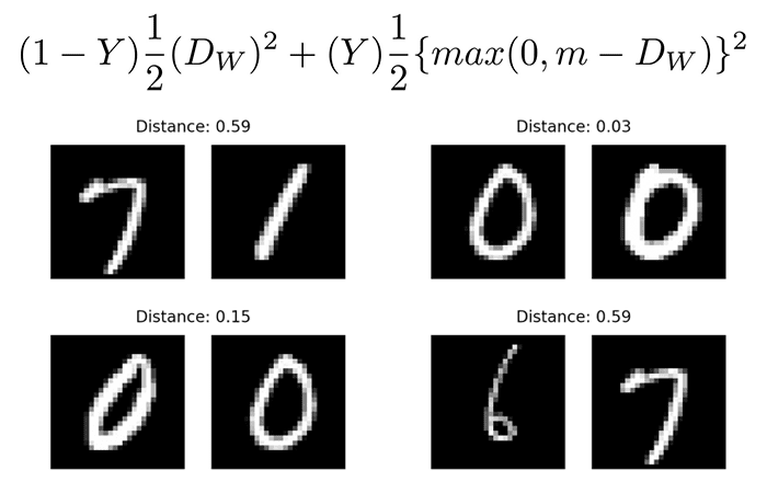
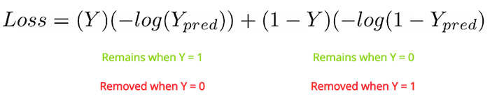
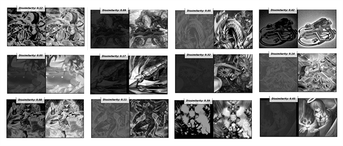
value is our label. It will be 1 if the image pairs are of the same class, and it will be 0 if the image pairs are of a different class.
  • The D_{w} 
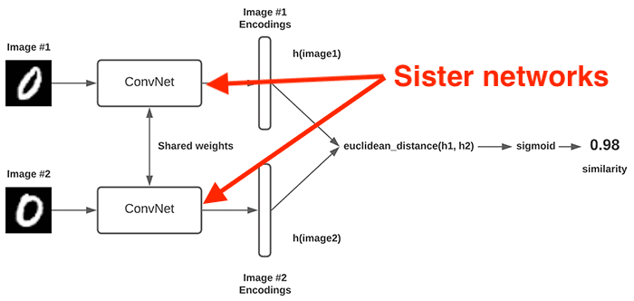
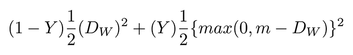
variable is the Euclidean distance between the outputs of the sister network embeddings.
  • The max function takes the largest value of 0 and the margin, m, minus the distance.

We’ll be implementing this loss function using Keras and TensorFlow later in this tutorial.

If you would like more mathematically motivated details on contrastive loss, be sure to refer to Hadsell et al.’s paper, Dimensionality Reduction by Learning an Invariant Mapping.

Configuring your development environment

This series of tutorials on siamese networks utilizes Keras and TensorFlow. If you intend on following this tutorial on the previous two parts in this series, I suggest you take the time now to configure your deep learning development environment.

You can utilize either of these two guides to install TensorFlow and Keras on your system:

Either tutorial will help you configure your system with all the necessary software for this blog post in a convenient Python virtual environment.

Having problems configuring your development environment?

Figure 3: Having trouble configuring your dev environment? Want access to pre-configured Jupyter Notebooks running on Google Colab? Be sure to join PyImageSearch Plus — you’ll be up and running with this tutorial in a matter of minutes.

All that said, are you:

  • Short on time?
  • Learning on your employer’s administratively locked system?
  • Wanting to skip the hassle of fighting with the command line, package managers, and virtual environments?
  • Ready to run the code right now on your Windows, macOS, or Linux system?

Then join PyImageSearch Plus today!

Gain access to Jupyter Notebooks for this tutorial and other PyImageSearch guides that are pre-configured to run on Google Colab’s ecosystem right in your web browser! No installation required.

And best of all, these Jupyter Notebooks will run on Windows, macOS, and Linux!

Project structure

Today’s tutorial on contrastive loss on siamese networks builds on my three previous tutorials that cover the fundamentals of building image pairs, implementing and training siamese networks, and using siamese networks for inference:

  1. Building image pairs for siamese networks with Python
  2. Siamese networks with Keras, TensorFlow, and Deep Learning
  3. Comparing images for similarity using siamese networks, Keras, and TensorFlow

We’ll be building on the knowledge we gained from those guides (including the project directory structure itself) today, so consider the previous guides required reading before continuing today.

Once you’ve gotten caught up, we can proceed to review our project directory structure:

$ tree . --dirsfirst
.
├── examples
│   ├── image_01.png
│   ├── image_02.png
│   ├── image_03.png
...
│   └── image_13.png
├── output
│   ├── contrastive_siamese_model
│   │   ├── assets
│   │   ├── variables
│   │   │   ├── variables.data-00000-of-00001
│   │   │   └── variables.index
│   │   └── saved_model.pb
│   └── contrastive_plot.png
├── pyimagesearch
│   ├── config.py
│   ├── metrics.py
│   ├── siamese_network.py
│   └── utils.py
├── test_contrastive_siamese_network.py
└── train_contrastive_siamese_network.py

6 directories, 23 files

Inside the pyimagesearch module you’ll find four Python files:

  1. config.py: Contains our configuration of important variables, including batch size, epochs, output file paths, etc.
  2. metrics.py: Holds our implementation of the contrastive_loss function
  3. siamese_network.py: Contains the siamese network model architecture
  4. utils.py: Includes helper utilities, including a function to generate image pairs, compute the Euclidean distance as a layer inside of a CNN, and a training history plotting function

We then have two Python driver scripts:

  1. train_contrastive_siamese_network.py: Trains our siamese neural network using contrastive loss and serializes the training history and model weights/architecture to disk inside the output directory
  2. test_contrastive_siamse_network.py: Loads our trained siamese network from disk and applies it to image pairs from inside the examples directory

Again, I cannot stress the importance of reviewing my previous series of tutorials on siamese networks. Doing so is an absolute requirement before continuing here today.

Implementing our configuration file

Our configuration file holds important variables used to train our siamese network with contrastive loss.

Open up the config.py file in your project directory structure, and let’s take a look inside:

# import the necessary packages
import os

# specify the shape of the inputs for our network
IMG_SHAPE = (28, 28, 1)

# specify the batch size and number of epochs
BATCH_SIZE = 64
EPOCHS = 100

# define the path to the base output directory
BASE_OUTPUT = "output"

# use the base output path to derive the path to the serialized
# model along with training history plot
MODEL_PATH = os.path.sep.join([BASE_OUTPUT,
	"contrastive_siamese_model"])
PLOT_PATH = os.path.sep.join([BASE_OUTPUT,
	"contrastive_plot.png"])

Line 5 sets our IMG_SHAPE dimensions. We’ll be working with the MNIST digits dataset, which has 28×28 grayscale (i.e., single channel) images.

We then set our BATCH_SIZE and number of EPOCHS to train before. These parameters were experimentally tuned.

Lines 16-19 define the output file paths for both our serialized model and training history.

For more details on the configuration file, refer to my tutorial on Siamese networks with Keras, TensorFlow, and Deep Learning.

Creating our helper utility functions

Figure 4: In order to train our siamese network, we need to generate positive and negative image pairs.

In order to train our siamese network model, we’ll need three helper utilities:

  1. make_pairs: Generates a set of image pairs from the MNIST dataset that will serve as our training set
  2. euclidean_distance: A custom layer implementation that computes the Euclidean distance between two volumes inside of a CNN
  3. plot_training: Plots the training and validation contrastive loss over the course of the training process

Let’s start off with our imports:

# import the necessary packages
import tensorflow.keras.backend as K
import matplotlib.pyplot as plt
import numpy as np

We then have our make_pairs function, which I discussed in detail in my Building image pairs for siamese networks with Python tutorial (make sure you read that guide before continuing):

def make_pairs(images, labels):
	# initialize two empty lists to hold the (image, image) pairs and
	# labels to indicate if a pair is positive or negative
	pairImages = []
	pairLabels = []

	# calculate the total number of classes present in the dataset
	# and then build a list of indexes for each class label that
	# provides the indexes for all examples with a given label
	numClasses = len(np.unique(labels))
	idx = [np.where(labels == i)[0] for i in range(0, numClasses)]

	# loop over all images
	for idxA in range(len(images)):
		# grab the current image and label belonging to the current
		# iteration
		currentImage = images[idxA]
		label = labels[idxA]

		# randomly pick an image that belongs to the *same* class
		# label
		idxB = np.random.choice(idx[label])
		posImage = images[idxB]

		# prepare a positive pair and update the images and labels
		# lists, respectively
		pairImages.append([currentImage, posImage])
		pairLabels.append([1])

		# grab the indices for each of the class labels *not* equal to
		# the current label and randomly pick an image corresponding
		# to a label *not* equal to the current label
		negIdx = np.where(labels != label)[0]
		negImage = images[np.random.choice(negIdx)]

		# prepare a negative pair of images and update our lists
		pairImages.append([currentImage, negImage])
		pairLabels.append([0])

	# return a 2-tuple of our image pairs and labels
	return (np.array(pairImages), np.array(pairLabels))

I’ve already covered this function in detail previously, but the gist here is that:

  1. In order to train siamese networks, we need examples of positive and negative image pairs
  2. A positive pair is two images that belong to the same class (i.e., two examples of the digit “8”)
  3. A negative pair is two images that belong to different classes (i.e., one image containing a “1” and the other image containing a “3”)
  4. The make_pairs function accepts an input set of images and associated labels and then constructs the positive and negative image pairs

The next function, euclidean_distance, accepts a 2-tuple of vectors and then computes the Euclidean distance between them, utilizing Keras/TensorFlow functions such that the Euclidean distance can be computed inside the siamese neural network:

def euclidean_distance(vectors):
	# unpack the vectors into separate lists
	(featsA, featsB) = vectors

	# compute the sum of squared distances between the vectors
	sumSquared = K.sum(K.square(featsA - featsB), axis=1,
		keepdims=True)

	# return the euclidean distance between the vectors
	return K.sqrt(K.maximum(sumSquared, K.epsilon()))

Finally, we have a helper utility, plot_training, which accepts a plotPath, plots our training and validation contrastive loss over the course of training, and then saves the plot to disk:

def plot_training(H, plotPath):
	# construct a plot that plots and saves the training history
	plt.style.use("ggplot")
	plt.figure()
	plt.plot(H.history["loss"], label="train_loss")
	plt.plot(H.history["val_loss"], label="val_loss")
	plt.title("Training Loss")
	plt.xlabel("Epoch #")
	plt.ylabel("Loss")
	plt.legend(loc="lower left")
	plt.savefig(plotPath)

Let’s move on to implementing the siamese network architecture itself.

Implementing our siamese network architecture

Figure 5: Siamese networks with Keras and TensorFlow.

Our siamese neural network architecture is essentially a basic CNN:

# import the necessary packages
from tensorflow.keras.models import Model
from tensorflow.keras.layers import Input
from tensorflow.keras.layers import Conv2D
from tensorflow.keras.layers import Dense
from tensorflow.keras.layers import Dropout
from tensorflow.keras.layers import GlobalAveragePooling2D
from tensorflow.keras.layers import MaxPooling2D

def build_siamese_model(inputShape, embeddingDim=48):
	# specify the inputs for the feature extractor network
	inputs = Input(inputShape)

	# define the first set of CONV => RELU => POOL => DROPOUT layers
	x = Conv2D(64, (2, 2), padding="same", activation="relu")(inputs)
	x = MaxPooling2D(pool_size=(2, 2))(x)
	x = Dropout(0.3)(x)

	# second set of CONV => RELU => POOL => DROPOUT layers
	x = Conv2D(64, (2, 2), padding="same", activation="relu")(x)
	x = MaxPooling2D(pool_size=2)(x)
	x = Dropout(0.3)(x)

	# prepare the final outputs
	pooledOutput = GlobalAveragePooling2D()(x)
	outputs = Dense(embeddingDim)(pooledOutput)

	# build the model
	model = Model(inputs, outputs)

	# return the model to the calling function
	return model

You can refer to my tutorial on Siamese networks with Keras, TensorFlow, and Deep Learning for more details on the model architecture and implementation.

Implementing contrastive loss with Keras and TensorFlow

With our helper utilities and model architecture implemented, we can move on to defining the contrastive_loss function in Keras/TensorFlow.

For reference, here is the equation for the contrastive loss function that we’ll be implementing in Keras/TensorFlow code:

Figure 6: Implementing the contrastive loss function with Keras and TensorFlow.

The full implementation of contrastive loss is concise, spanning only 18 lines, including comments:

# import the necessary packages
import tensorflow.keras.backend as K
import tensorflow as tf

def contrastive_loss(y, preds, margin=1):
	# explicitly cast the true class label data type to the predicted
	# class label data type (otherwise we run the risk of having two
	# separate data types, causing TensorFlow to error out)
	y = tf.cast(y, preds.dtype)

	# calculate the contrastive loss between the true labels and
	# the predicted labels
	squaredPreds = K.square(preds)
	squaredMargin = K.square(K.maximum(margin - preds, 0))
	loss = K.mean(y * squaredPreds + (1 - y) * squaredMargin)

	# return the computed contrastive loss to the calling function
	return loss

Line 5 defines our contrastive_loss function, which accepts three arguments, two of which are required and the third optional:

  1. y: The ground-truth labels from our dataset. A value of 1 indicates that the two images in the pair are of the same class, while a value of 0 indicates that the images belong to two different classes.
  2. preds: The predictions from our siamese network (i.e., distances between the image pairs).
  3. margin: Margin used for the contrastive loss function (typically this value is set to 1).

Line 9 ensures our ground-truth labels are of the same data type as our preds. Failing to perform this explicit casting may result in TensorFlow erroring out when we try to perform mathematical operations on y and preds.

We then proceed to compute the contrastive loss by:

  1. Taking the square of the preds (Line 13)
  2. Computing the squaredMargin, which is the square of the maximum value of either 0 or margin - preds (Line 14)
  3. Computing the final loss (Line 15)

The computed contrastive loss value is then returned to the calling function.

I suggest you review the “What is contrastive loss? And how can contrastive loss be used to train siamese networks?” section above and compare our implementation to the equation so you can better understand how contrastive loss is implemented.

Creating our contrastive loss training script

We are now ready to implement our training script! This script is responsible for:

  1. Loading the MNIST digits dataset from disk
  2. Preprocessing it and constructing image pairs
  3. Instantiating the siamese neural network architecture
  4. Training the siamese network with contrastive loss
  5. Serializing both the trained network and training history plot to disk

The majority of this code is identical to our previous post on Siamese networks with Keras, TensorFlow, and Deep Learning, so while I’m still going to cover our implementation in full, I’m going to defer a detailed discussion to the previous post (and of course, pointing out the details along the way).

Open up the train_contrastive_siamese_network.py file in your project directory structure, and let’s get to work:

# import the necessary packages
from pyimagesearch.siamese_network import build_siamese_model
from pyimagesearch import metrics
from pyimagesearch import config
from pyimagesearch import utils
from tensorflow.keras.models import Model
from tensorflow.keras.layers import Dense
from tensorflow.keras.layers import Input
from tensorflow.keras.layers import Lambda
from tensorflow.keras.datasets import mnist
import numpy as np

Lines 2-11 import our required Python packages. Note how we are importing the metrics submodule of pyimagesearch, which contains our contrastive_loss implementation.

From there we can load the MNIST dataset from disk:

# load MNIST dataset and scale the pixel values to the range of [0, 1]
print("[INFO] loading MNIST dataset...")
(trainX, trainY), (testX, testY) = mnist.load_data()
trainX = trainX / 255.0
testX = testX / 255.0

# add a channel dimension to the images
trainX = np.expand_dims(trainX, axis=-1)
testX = np.expand_dims(testX, axis=-1)

# prepare the positive and negative pairs
print("[INFO] preparing positive and negative pairs...")
(pairTrain, labelTrain) = utils.make_pairs(trainX, trainY)
(pairTest, labelTest) = utils.make_pairs(testX, testY)

Line 15 loads the MNIST dataset with the pre-supplied training and testing splits.

We then preprocess the dataset by:

  1. Scaling the input pixel intensities in the images from the range [0, 255] to [0, 1] (Lines 16 and 17)
  2. Adding a channel dimension (Lines 20 and 21)
  3. Constructing our image pairs (Lines 25 and 26)

Next, we can instantiate the siamese network architecture:

# configure the siamese network
print("[INFO] building siamese network...")
imgA = Input(shape=config.IMG_SHAPE)
imgB = Input(shape=config.IMG_SHAPE)
featureExtractor = build_siamese_model(config.IMG_SHAPE)
featsA = featureExtractor(imgA)
featsB = featureExtractor(imgB)

# finally, construct the siamese network
distance = Lambda(utils.euclidean_distance)([featsA, featsB])
model = Model(inputs=[imgA, imgB], outputs=distance)

Lines 30-34 create our sister networks:

  • We start by creating two inputs, one for each image in the image pair (Lines 30 and 31).
  • We then build the sister network architecture, which acts as our feature extractor (Line 32).
  • Each image in the pair will be passed through our feature extractor, resulting in a vector that quantifies each image (Lines 33 and 34).

Using the 48-d vector generated by the sister networks, we proceed to compute the euclidean_distance between our two vectors (Line 37) — this distance serves as our output from the siamese network:

  • The smaller the distance is, the more similar the two images are.
  • The larger the distance is, the less similar the images are.

Line 38 defines the model by specifying imgA and imgB, our two images in the image pair, as inputs, and our distance layer as the output.

Finally, we can train our siamese network using contrastive loss:

# compile the model
print("[INFO] compiling model...")
model.compile(loss=metrics.contrastive_loss, optimizer="adam")

# train the model
print("[INFO] training model...")
history = model.fit(
	[pairTrain[:, 0], pairTrain[:, 1]], labelTrain[:],
	validation_data=([pairTest[:, 0], pairTest[:, 1]], labelTest[:]),
	batch_size=config.BATCH_SIZE,
	epochs=config.EPOCHS)

# serialize the model to disk
print("[INFO] saving siamese model...")
model.save(config.MODEL_PATH)

# plot the training history
print("[INFO] plotting training history...")
utils.plot_training(history, config.PLOT_PATH)

Line 42 compiles our model architecture using the contrastive_loss function.

We then proceed to train the model using our training/validation image pairs (Lines 46-50) and then serialize the model to disk (Line 54) and plot the training history (Line 58).

Training a siamese network with contrastive loss

We are now ready to train our siamese neural network with contrastive loss using Keras and TensorFlow.

Make sure you use the “Downloads” section of this guide to download the source code, helper utilities, and contrastive loss implementation.

From there, you can execute the following command:

$ python train_contrastive_siamese_network.py
[INFO] loading MNIST dataset...
[INFO] preparing positive and negative pairs...
[INFO] building siamese network...
[INFO] compiling model...
[INFO] training model...
Epoch 1/100
1875/1875 [==============================] - 81s 43ms/step - loss: 0.2038 - val_loss: 0.1755
Epoch 2/100
1875/1875 [==============================] - 80s 43ms/step - loss: 0.1756 - val_loss: 0.1571
Epoch 3/100
1875/1875 [==============================] - 80s 43ms/step - loss: 0.1619 - val_loss: 0.1394
Epoch 4/100
1875/1875 [==============================] - 81s 43ms/step - loss: 0.1548 - val_loss: 0.1356
Epoch 5/100
1875/1875 [==============================] - 81s 43ms/step - loss: 0.1501 - val_loss: 0.1262
...
Epoch 96/100
1875/1875 [==============================] - 81s 43ms/step - loss: 0.1264 - val_loss: 0.1066
Epoch 97/100
1875/1875 [==============================] - 80s 43ms/step - loss: 0.1262 - val_loss: 0.1100
Epoch 98/100
1875/1875 [==============================] - 82s 44ms/step - loss: 0.1262 - val_loss: 0.1078
Epoch 99/100
1875/1875 [==============================] - 81s 43ms/step - loss: 0.1268 - val_loss: 0.1067
Epoch 100/100
1875/1875 [==============================] - 80s 43ms/step - loss: 0.1261 - val_loss: 0.1107
[INFO] saving siamese model...
[INFO] plotting training history...
Figure 7: Training our siamese network with contrastive loss.

Each epoch took ~80 seconds on my 3 GHz Intel Xeon W processor. Training would be even faster with a GPU.

Our training history can be seen in Figure 7. Notice how our validation loss is actually lower than our training loss, a phenomenon that I discuss in this tutorial.

Having our validation loss lower than our training loss implies that we can “train harder” to improve our siamese network accuracy, typically by relaxing regularization constraints, deepening the model, and using a more aggressive learning rate.

But for now, our training model is more than sufficient.

Implementing our contrastive loss test script

The final script we need to implement is test_contrastive_siamese_network.py. This script is essentially identical to the one covered in our previous tutorial on Comparing images for similarity using siamese networks, Keras, and TensorFlow, so while I’ll still cover the script in its entirety today, I’ll defer a detailed discussion to my previous guide.

Let’s get started:

# import the necessary packages
from pyimagesearch import config
from pyimagesearch import utils
from tensorflow.keras.models import load_model
from imutils.paths import list_images
import matplotlib.pyplot as plt
import numpy as np
import argparse
import cv2

Lines 2-9 import our required Python packages.

We’ll be using load_model to load our serialized siamese network from disk. The list_images function will be used to grab image paths and facilitate building sample image pairs.

Let’s move on to our command line arguments:

# construct the argument parser and parse the arguments
ap = argparse.ArgumentParser()
ap.add_argument("-i", "--input", required=True,
	help="path to input directory of testing images")
args = vars(ap.parse_args())

The only command line argument we need is --input, the path to our directory containing sample images we want to build pairs from (i.e., the examples directory in our project directory).

Speaking of building image pairs, let’s do that now:

# grab the test dataset image paths and then randomly generate a
# total of 10 image pairs
print("[INFO] loading test dataset...")
testImagePaths = list(list_images(args["input"]))
np.random.seed(42)
pairs = np.random.choice(testImagePaths, size=(10, 2))

# load the model from disk
print("[INFO] loading siamese model...")
model = load_model(config.MODEL_PATH, compile=False)

Line 20 grabs the paths to all images in our --input directory. We then randomly generate a total of 10 pairs of images (Line 22).

Line 26 loads our trained siamese network from disk.

With the siamese network loaded from disk, we can now compare images:

# loop over all image pairs
for (i, (pathA, pathB)) in enumerate(pairs):
	# load both the images and convert them to grayscale
	imageA = cv2.imread(pathA, 0)
	imageB = cv2.imread(pathB, 0)

	# create a copy of both the images for visualization purpose
	origA = imageA.copy()
	origB = imageB.copy()

	# add channel a dimension to both the images
	imageA = np.expand_dims(imageA, axis=-1)
	imageB = np.expand_dims(imageB, axis=-1)

	# add a batch dimension to both images
	imageA = np.expand_dims(imageA, axis=0)
	imageB = np.expand_dims(imageB, axis=0)

	# scale the pixel values to the range of [0, 1]
	imageA = imageA / 255.0
	imageB = imageB / 255.0

	# use our siamese model to make predictions on the image pair,
	# indicating whether or not the images belong to the same class
	preds = model.predict([imageA, imageB])
	proba = preds[0][0]

Line 29 loops over all pairs. For each pair, we:

  1. Load the two images from disk (Lines 31 and 32)
  2. Clone the images such that we can visualize/draw on them (Lines 35 and 36)
  3. Add a channel dimension to both images, a requirement for inference (Lines 39 and 40)
  4. Add a batch dimension to the images, again, a requirement for inference (Lines 43 and 44)
  5. Scale the pixel intensities from the range [0, 255] to [0, 1], just like we did during training

The image pairs are then passed through our siamese network on Lines 52 and 53, resulting in the computed Euclidean distance between the vectors generated by the sister networks.

Again, keep in mind that the smaller the distance is, the more similar the two images are. Conversely, the larger the distance, the less similar the images are.

The final code block handles visualizing the two images in the pair along with their computed distance:

	# initialize the figure
	fig = plt.figure("Pair #{}".format(i + 1), figsize=(4, 2))
	plt.suptitle("Distance: {:.2f}".format(proba))

	# show first image
	ax = fig.add_subplot(1, 2, 1)
	plt.imshow(origA, cmap=plt.cm.gray)
	plt.axis("off")

	# show the second image
	ax = fig.add_subplot(1, 2, 2)
	plt.imshow(origB, cmap=plt.cm.gray)
	plt.axis("off")

	# show the plot
	plt.show()

Congratulations on implementing an inference script for siamese networks! For more details on this implementation, refer to my previous tutorial, Comparing images for similarity using siamese networks, Keras, and TensorFlow.

Making predictions using our siamese network with contrastive loss model

Let’s put our test_contrastive_siamse_network.py script to work. Make sure you use the “Downloads” section of this tutorial to download the source code, pre-trained model, and example images.

From there, you can run the following command:

$ python test_contrastive_siamese_network.py --input examples
[INFO] loading test dataset...
[INFO] loading siamese model...
Figure 8: Results of applying our siamese network inference script. Image pairs with smaller distances are considered to belong to the same class, while image pairs with larger distances belong to different classes.

Looking at Figure 8, you’ll see that we have sets of example image pairs presented to our siamese network trained with contrastive loss.

Images that are of the same class have lower distances while images of different classes have larger classes.

You can thus set a threshold value, T, to act as a cutoff on distance. If the computed distance, D, is < T, then the image pair must belong to the same class. Otherwise, if D >= T, then the images are different classes.

Setting the threshold T should be done empirically through experimentation:

  • Train the network.
  • Compute distances for image pairs.
  • Manually visualize the pairs and their corresponding differences.
  • Find a cutoff value that maximizes correct classifications and minimizes incorrect ones.

In this case, setting T=0.16 would be an appropriate threshold, since it allows us to correctly mark all image pairs that belong to the same class, while all image pairs of different classes are treated as such.

What’s next?

Figure 9: If you want a comprehensive education in deep learning, pick up a copy of Deep Learning for Computer Vision with Python. My team and I will be there to support you as you dive into the material and start to implement it.

If you’re interested in learning more about siamese neural networks, I strongly recommend that you start with the fundamentals of deep learning and computer vision.

You’ll find it much easier to implement these advanced neural network architectures if you have a thorough understanding of the basics.

My book Deep Learning for Computer Vision with Python blends theory with code implementation, so you’ll build a strong foundation for your computer vision, deep learning, and artificial intelligence education.

Inside this book you learn:

  • Everything you need to know about the fundamentals and theory of deep learning without unnecessary mathematical jargon. You’ll be able to understand and implement the basic equations easily because they are all backed up with code walkthroughs. You definitely don’t need a degree in advanced math to understand this book.
  • How to implement state-of-the-art custom neural network architectures and create your own. By the end of the book, you’ll thoroughly understand how to implement CNNs such as ResNet, SqueezeNet, etc., and you’ll be confident to create custom neural network architectures.
  • How to train CNNs on your own datasets. Unlike most deep learning tutorials, in this book you’ll learn how to work with your own custom datasets. In fact. you’ll be training CNNs on your own datasets even before you finish the book.
  • Object detection (Faster R-CNNs, Single Shot Detectors, and RetinaNet) and instance segmentation (Mask R-CNN). You’ll learn how to create your own custom object detectors and segmentation networks.

You’ll also find answers and proven code recipes to:

  • Create and prepare your own custom image datasets for image classification, object detection, and segmentation
  • Understand the algorithms behind deep learning for computer vision and their implementations by getting real-life experience from hands-on tutorials
  • Maximize the accuracy of your models by taking action with my tips and best practices

This book is packed full of highly actionable content and is delivered in the same no-nonsense teaching style you expect from PyImageSearch. If you’d like to try before you buy, click here and I’ll send you the full table of contents and some sample chapters.

Wondering how far you can go with deep learning? Check out these success stories from students who decided to take a deep dive into deep learning and computer vision.

Summary

In this tutorial you learned about contrastive loss, including how it’s a better loss function than binary cross-entropy for training siamese networks.

What you need to keep in mind here is that a siamese network isn’t specifically designed for classification. Instead, it’s utilized for differentiation, meaning that it should not only be able to tell if an image pair belongs to the same class or not but whether the two images are identical/similar or not.

Contrastive loss works far better in this situation.

I recommend you experiment with both binary cross-entropy and contrastive loss when training your own siamese neural networks, but I think you’ll find that overall, contrastive loss does a much better job.

To download the source code to this post (and be notified when future tutorials are published here on PyImageSearch), simply enter your email address in the form below!

Download the Source Code and FREE 17-page Resource Guide

Enter your email address below to get a .zip of the code and a FREE 17-page Resource Guide on Computer Vision, OpenCV, and Deep Learning. Inside you'll find my hand-picked tutorials, books, courses, and libraries to help you master CV and DL!

The post Contrastive Loss for Siamese Networks with Keras and TensorFlow appeared first on PyImageSearch.


Using computer vision and OCR for immigration document classification (an interview with Vince DiMascio)

$
0
0

In this post, I interview Vince DiMascio, CIO/CTO of Berry Appleman & Leiden (BAL), a law firm specializing in corporate immigration.

BAL is using computer vision, machine learning, and artificial intelligence to automatically classify immigration documents, thus helping expedite the arduous task of gathering and validating documents.

Recently, Vince, along with Dr. Tim Oates (my former PhD advisor) published a paper on their work, Immigration Document Classification and Automated Response Generation. This work was a joint effort between BAL and Synaptiq, which Dr. Oates co-founded with his partner, Stephen Sklarew.

Today we’re going to sit down with Vince and discuss their paper, including how their techniques can help immigration teams be more efficient, run with less overhead, and ensure their clients are successful.

An interview with Vince DiMascio, CIO and CTO at Berry Appleman & Leiden (BAL)

Adrian: Hi, Vince! Thank you for being here on the PyImageSearch blog. I know you’re very busy as the CIO of Berry Appleman & Leiden (BAL). We all appreciate you taking the time to be here.

Vince: Thank you for having me. It’s great to chat with you, Adrian.


Adrian: Can you tell us a bit about yourself and your role at BAL?

Vince: I’m the CIO and CTO for BAL. We are a global corporate immigration law firm. We’ve been around for 40 years. Technology has always been central to how we operate and serve our clients.

I joined the firm about five years ago to set the technology strategy and lead the teams to execute it. In my role, I handle anything and everything related to technology. Those duties range from desktop support to Artificial Intelligence (AI) and automation, professional services teams, and a digital products organization that handles the development and introduction of cutting edge products.


Adrian: I’m curious, given that you work for a law firm, how did you first become interested in computer vision and machine learning?

Vince: I happened to be lucky enough to bring the right skills to the right place at the right time.

Before BAL, I was in consulting. I was frequently involved with law firms’ and legal departments’ use of technology. I started looking at machine learning when the federal rules changed in the early 2000s, really giving birth to e-discovery. Back then, we were using machine learning to do things like concept clustering, natural language processing, and even predictive coding to find relevant documents and expedite discovery. That work set me on course to help businesses by responsibly applying cutting edge technology in heavily regulated and high stakes environments.

When I came to BAL, we set our 2020 strategy. We knew we could do a lot for our clients by using data well, applying machine learning, and bringing those together with great design to deliver unmatched products, insights, and experiences. Like litigation, immigration law can be paper-heavy, so I knew we could make an impact by handling unstructured data, optimizing legal workflows with technology, and leveraging AI. That includes developing and operationalizing systems that use computer vision and machine learning.


Adrian: How did you find out about PyImageSearch?

Vince: When we started looking at this as an opportunity, that’s when I found PyImageSearch. I was looking for ways to classify images of documents to sort them out and route them down different workflow paths, including extracting information. For example, a passport could go down a certain path and have information extracted from its machine readable zone area. But a government form might go down a different path, to have a different extraction approach. My searching led me to PyImageSearch, a treasure trove of information, code, and community around computer vision. It helped us as we continued to look at how we could leverage CV internally with BAL. We’ve been subscribers to the PyImageSearch community ever since.


Figure 1: Distinguishing Between RPA and IA

Adrian: What was your experience like working with PyImageSearch’s consulting partner, Synaptiq? Why did you choose to work with them instead of using packaged Artificial Intelligence (AI) and Robotic Processing Automation (RPA) solutions?

Vince: The experience has been outstanding, and that’s why we remain a client. Synaptiq works as partners with us rather than as a traditional vendor. They focus on understanding the problems and opportunities we’re facing. They team up with our legal, data, and products staff to develop solutions with us that we can drive together. We chose them rather than leveraging packaged solutions. We found that, while packaged AI and RPA are good at a lot of things, they’re not great in our focused areas. And we need to be the best at that narrower set of things that we do. Since we’re in uncharted territory on the things we’re doing, it sometimes makes sense to build. We do leverage packaged solutions where appropriate for commodity work. We engineer it ourselves in the areas where we need to deliver unique, exceptional value through new technology.

When you’re doing that, it’s essential to team up with a partner who has years of data science, machine learning, and computer vision skills across various industries and determine which model to use, which approach to follow, or what framework. Beyond that, we need to decide how we structure our teams, deliver the model, and operationalize it. It’s one thing to do it in a lab. We see that lab model everywhere, especially these days in legal. But to truly bring AI into a business and operationalize it, you need strong business alignment and the right technology capabilities.


Adrian: You and Synaptiq recently published a paper on using computer vision and OCR to automatically process and prepare supporting documents for the United States visa petitions presented at the IEEE / MLLD 2020 International Workshop on Mining and Learning in the Legal Domain in November. Can you explain what MLLD is and why it’s important for legal professionals with scientific backgrounds?

Vince: First, I’d like to clarify what the project is. The system provides our clients with a second set of eyes to help with some of the rote work performed in connection with immigration case processing. The system doesn’t independently automatically process and prepare documents. It enhances quality and turnaround time by classifying documents we receive in the mail. Then it reads those documents to identify what’s being requested. A final step passes that information to a system that works like a copy-paste action to create a draft that a legal professional can use to start the legal work.

This is important for legal professionals, so it was selected to be presented at IEEE-MLLD. It’s truly machine learning, and it’s applicable beyond immigration law. One example of another context is in handling a third-party subpoena. In that context, one party receives a request for documents. The third-party will carefully read the request, identify what’s being requested, and often serve written objections to those requests. So in a similar workflow, this technology would help such third parties see that they’ve identified and addressed what’s being requested, using approved standard form templates and content.


Figure 2: “Smart OCR”: High-performing ML system can handle images and text in ways that go well beyond OCR and can evolve.

Adrian: What is the typical sequence of events when a prospective employee applies for a U.S. work visa? I imagine a lot of documents are generated and that there is an extensive paper trail.

Vince: The process can be paper-intensive, which is why it’s important to have high performing accurate machine learning systems that can handle documents and document images in ways that go well beyond OCR, and that can evolve. I’m not an attorney, and the process varies to some extent, depending on the visa type and circumstances. I think of the process in a few phases: intake, preparation, filing, and decision.

First, there’s an “intake” process where you collect the materials you’ll need to file a petition. This is a range of documents and forms, some of which are collected electronically as PDF, Word, or image files. When you have the material you need, you move into the “prepare” phase, where you fill out various forms, some online, some as PDF files. In this phase, you assemble the information into a particular filing order. When the materials are ready, you move to the “filing” phase, where you perform a final review and then file it with the agency, usually with a check for filing fees. At that point, it’s with the government, and you start monitoring the status of the filing. That’s when the United States Citizenship and Immigration Services (USCIS) might send a Request for Evidence (RFE), which is the type of document we trained machine learning systems to classify and read. USCIS will send RFEs when they don’t have enough information to decide the petition. So if you receive an RFE, you’ll need to address it. Eventually, you end up at the “decision” phase, where you get a decision from USCIS.


Adrian: What is an RFE, and how commonplace is this with each job candidate?

Vince: An RFE is a Request for Evidence, which is a request for additional information that the government wants from the foreign national to determine if the application is approved or not. It could be just a missing document, or it could be something that takes more effort to respond to.


Adrian: Tell us about how you came up with the idea of using computer vision and OCR with this process?

Vince: This idea came from our innovation pipeline. We have functions dedicated to defining, piloting, and scaling AI use cases. Unlike the “lab” model we’ve seen repeatedly fail across industries, we embed innovation and AI directly in our business, so we’re aligned with our clients’ needs. We have a formal innovation program where we invite employees and leaders at every level to join and take part in creating new solutions to firm administrative and client challenges alike. Our technical and products teams review and evaluate the ideas in terms of viability and value. We use product management methodology to back into the actual problem and see if we can generalize it to the greatest extent possible. Then we sprint and iterate. This original idea came through that pipeline, and once we evaluated it as a concept, it made sense to do it.


Adrian: You mentioned different phases: Intake, Preparation, Filing, and feeding various documents into those processes. So the system you are developing can differentiate between the document types?

Vince: That’s a good question. On our side, we receive material through a variety of secure channels. The materials are often PDF files, scanned images, or a picture taken from a mobile device. We get an image of this document; it’s fixed, it’s a grid of pixels, and we need to turn that into information we can use. We have to transcribe that image into text information and sometimes put it into a government form. We use novel automated methods to provide high-quality data services and an exceptional experience to our clients. As a simple example, when a foreign national uploads an image of a passport, they don’t have to type in the text. It’s extracted automatically and placed into fields for them. We have automation like that throughout the journey to enhance quality and experience.


Figure 3: First of its kind AI ensemble: Image and text classifier work in concert to categorize documents according to their visual and language content. Text is extracted from RFE documents and trained classifier to identify types of evidence requested by USCIS.

Adrian: Can you give us a high-level overview of the system you and Synaptiq developed?

Vince: We created two systems that work well independently and together.

The first system classifies document images common in U.S. work visa petitions. So you can submit a document image to our service, and the service will tell you the type of document you submitted. For example, a passport, a birth certificate, a certain government form, or an RFE. That system alone helps label or sort documents or priming a downstream text extraction system to know what to look for and where to look when extracting the relevant text.

The second system reads RFEs, which are the letters I mentioned earlier. RFEs are issued by the USCIS when it needs more information to decide on an application. You can post the RFE letter to this second system, and it will read the letter and then respond with a list of what additional information the USCIS is asking for in the RFE. Used together, we can give our people and our clients an extra set of eyes to drive quality throughout the paper handling process. This also allows us to catalog the types of government requests and what combination of factors is most likely to give rise to them.

Figure 4: Our System: Applying the Reusable Framework.

The text extraction components embedded in the classifier and the RFE reader are the systems’ unsung heroes. Machine learning techniques, such as those used to remove noise, deskew, or leverage custom language models to get text extraction right, are critical to achieving high-quality results. All of that is available in PyImageSearch books for understanding, code for delivering, and VMs to run it.


Adrian: On the initial application processing, how accurate is the first pass, and what type of QC is recommended for the attorneys to conduct?

Vince: It’s really important to reiterate that nothing works independently and autonomously here. We have humans in the loop on every step of this, given the stakes. Empirical results suggest that our approach achieves considerable accuracy.

Our attorneys aren’t QCing. They’re doing the legal work. The systems are double-checking materials handled and generated in connection with that work, so we add another layer of review and the second set of hands to the operation. It gives our people “superpowers.”


Adrian: During the initial application processing, does your method gather data and fill out forms on the attorney’s behalf, or does it also detect potential issues or points of contention (for example, would it flag if a passport is set to expire or if there appears to be a gap in the individual’s work authorization?)

Vince: That’s a great question because this solution isn’t filling out forms. First, it’s classifying documents. If it finds an RFE, it then can read the text from the letter, interpret the text, and select a specifically curated form template for the attorney to use. It can also merge some data into the document from our case management system, just like Microsoft Word or Google Docs does, but it’s not drafting a response. We have other data health mechanisms in the filing process that address the date-related issues you’re referencing.


Adrian: Can your solution be used on all RFEs, or does it need to be trained on the specific RFE type first?

Vince: It’s flexible. An RFE typically is based on a template USCIS provides its officers as a starting point. The officers customize the RFE based on the application. So we maintain a table of RFE reasons for each type of RFE, and when we send the letter to the system, we also tell the system what kind of visa it is. And it uses that information to determine which set of known reasons to use in the language model. Again, we could just as easily load a table of common subpoena requests and their classifications and use it for a subpoena response process.


Adrian: For the more complex RFE, such as the specialty occupation RFE, how does this generate the initial response for the lawyer to review and edit? What documents is it pulling from to counter the RFE? And for this RFE type specifically, how “complete” is the first draft of the response to the human attorneys?

Vince: Just like USCIS, we maintain model documents, which are standard form templates that have placeholders for address, salutation, formatting, standard paragraphs, and that sort of thing. There’s a standard mail-merge to insert data such as the client company name, foreign national name, etc., that’s been around for a long time. That’s all there is related to the use of templates. The attorney authors the response’s substance. It’s just creating a skeleton from where the human starts regarding the completeness. You can think of it as a more “enhanced draft,” along with a list of what’s being requested.


Adrian: How does the machine taking care of the repetitive administrative work allow the attorney to focus on more time-intensive and specialized legal work for their client?

Vince: The system adds additional reviewers to drive the work quality. And so, the real business value of this tool is a greater, perhaps more robust response than you might get from another firm without a subsequent set of eyes to catch every nuance. We can also drive analytics that inform the legal strategy underlying the response language. The goal is to create a virtuous cycle in which we constantly improve our responses to ever-shifting government requests and do so in the most efficient way possible. Then we merge data from our databases into the templates, which is standard practice.


Adrian: How does your solution help BAL, and more importantly, how does it help your clients be more successful?

Vince: Given that it’s enhancing the quality of our work specifically around RFEs and on the intake side, it allows us to capture and label more information to see the trends in the attacks for a particular occupation, for particular industries, or more broadly. This helps us deliver valuable talent management insights to our clients.


Adrian: What are your next steps with the project? Are you continuing to develop and refine the system?

Vince: We’re going to keep running it, training it, and finding ways to deliver value to our clients with it. The idea is, if we know everything about RFE volume, what’s in the letters, what if there’s seasonality or spikes, etc., we can have that information at hand right away to advise our clients. Our clients want data-driven insights as part of our services. The days of anecdotes are in the past.


Adrian: Is there any advice you would give to someone who wants to follow in your footsteps, learn computer vision and deep learning, and then publish a paper or do work in the legal space?

Vince: Pick a project that you care about and start building. Sign up for PyImageSearch, and go through the training available there, get the books, sign up for the community, begin to collaborate there. It’s a tremendously valuable set of resources and a large active community. The resources are accelerators to understanding, developing, and deploying these capabilities. And documents are probably the most boring chapters. There are lessons and code about handling streaming video, photos, license plates, wild animals, detective surveillance to find out who is stealing beer from your refrigerator. It’s amazing, accessible, practical, and fun. Find something that has business value, be scientific about executing it, and take the time to write it down. Applied AI is still rare, despite all the hype you hear about it, so if you build something and use it, your chances of getting accepted to a major and prestigious conference like this may be better than you think.


Adrian: What’s next for BAL and AI in 2021?

Vince: It’s about pushing the envelope and continuing to lead our industry in how we deliver technology, experience, and insights for our clients. That means embedding intelligence everywhere as we evolve our AI-first operating model. And to do that, we’re growing our technology, product, and design teams to maintain the distance we have from our competitors.

An interesting area of pursuit is leveraging AI without undermining the attorney-client relationship’s importance. Human interaction is fundamental to the work we do. So we enhance the quality and speed with which we help our clients answer questions, queries, problem resolution, and see that data interaction occurs, so it’s not an impediment. We also use AI to enable our professionals to deliver legal services than any other firm better.

BAL has always led the industry in terms of technology innovation. For a few examples, just this year, we were awarded Best Legal Solution for our Cobalt digital platform, an IDG CIO 100 award for our tech teams, and a Business Transformation 150 award from Constellation Research for our work in innovating. We will continue to deliver cutting-edge technology-enabled services and digital products that globally power human achievement.


Adrian: If a PyImageSearch reader wants to go through the paper, where can they find it?

Vince: You can download a PDF of the paper from arXiv here: https://arxiv.org/abs/2010.01997


Adrian: Excellent. Congrats again on the paper, and thank you for taking the time to chat with me today. I look forward to keeping in touch.

Vince: Thank you, Adrian, me too. Looking forward to chatting with you again soon.

Summary

In this blog post, we interviewed Vince DiMascio, CIO/CTO of Berry Appleman & Leiden (BAL), a law firm specializing in corporate immigration.

BAL has recently worked with Synaptiq, an artificial intelligence consulting company cofounded by my former PhD advisor, Dr. Tim Oates.

Together, BAL and Synaptiq have published a paper on automatic immigration document classification, a system that allows immigration firms to be more efficient when responding to Request for Evidence (RFEs) from the US government.

Their system is a success, demonstrating how AI can be applied to nearly every field in the world.

If you’re interested in working with Synaptiq and seeing how artificial intelligence can be leveraged to make your company more efficient and profitable, just fill out this form for a free initial consultation.


PyImageSearch Consulting Services

I’ve teamed up with my former PhD advisor, Dr. Tim Oates, and Stephen Sklarew, a product and technology executive consultant, to offer PyImageSearch Consulting for Computer Vision, Deep Learning, and Artificial Intelligence through Synaptiq.

Founded in 2015, Synaptiq is a full-scale artificial intelligence consultancy with over 40 clients in more than 20 sectors worldwide. Our seasoned team of experts, including 16 Data Scientists (6 with PhDs), partner directly with each client to identify and deliver impactful solutions to real-world problems AI solves best.

If you are interested in working with Synaptiq, the consulting firm Vince DiMascio collaborated with on this solution (and PyImageSearch’s official consulting partner), use this link to tell us more about your project.

We look forward to hearing from you and learning more about your project.

The post Using computer vision and OCR for immigration document classification (an interview with Vince DiMascio) appeared first on PyImageSearch.

Adversarial attacks with FGSM (Fast Gradient Sign Method)

$
0
0

In this tutorial, you will learn how to perform adversarial attacks using the Fast Gradient Sign Method (FGSM). We will implement FGSM using Keras and TensorFlow.

Previously, we learned how to implement two forms of adversarial image attacks:

  1. Untargeted adversarial attacks, where we cannot control the output label of the adversarial image.
  2. Targeted adversarial attacks, where we can control the output label of the image.

Today we’re going to look at another untargeted adversarial image generation method called the Fast Gradient Sign Method (FGSM). As you’ll see, this method is super easy to implement.

Then, in the next two weeks, you’ll learn how to defend against adversarial attacks by updating your training procedure to utilize FGSM, thereby improving the accuracy and robustness of your model.

To learn how to perform adversarial attacks with the Fast Gradient Sign Method, just keep reading.

Looking for the source code to this post?

Jump Right To The Downloads Section

Adversarial attacks with FGSM (Fast Gradient Sign Method)

In the first part of this tutorial, you’ll learn about the Fast Gradient Sign Method and its use for adversarial image generation.

From there, we’ll configure our development environment and review our project directory structure.

We’ll then implement three Python scripts:

  1. The first one will contain SimpleCNN, our implementation of a basic CNN that we’ll train on the MNIST dataset.
  2. Our second Python script will contain our implementation of the FGSM for adversarial image generation.
  3. Finally, our third script will train our CNN on MNIST and then demonstrate how to use FGSM to fool our trained CNN into making incorrect predictions.

If you haven’t yet, I recommend that you read my previous two tutorials on adversarial image generation:

  1. Adversarial images and attacks with Keras and TensorFlow
  2. Targeted adversarial attacks with Keras and TensorFlow

These two guides are considered required reading as I’ll be assuming you already know the basics of adversarial image generation. If you haven’t read those tutorials yet, I suggest you stop now and read them first.

The Fast Gradient Sign Method (FGSM)

Figure 1: The Fast Gradient Sign Method (FGSM) for adversarial image generation (image source).

The Fast Gradient Sign Method (FGSM) is a simple yet effective method to generate adversarial images. First introduced by Goodfellow et al. in their paper, Explaining and Harnessing Adversarial Examples, FGSM works by:

  1. Taking an input image
  2. Making predictions on the image using a trained CNN
  3. Computing the loss of the prediction based on the true class label
  4. Calculating the gradients of the loss with respect to the input image
  5. Computing the sign of the gradient
  6. Using the signed gradient to construct the output adversarial image

This process may sound complicated, but as you’ll see, we’ll be able to implement the entire FGSM function in under 30 lines of code (including comments).

How does the Fast Gradient Sign Method work?

The FGSM exploits the gradients of a neural network to build an adversarial image, similar to what we’ve done in the untargeted adversarial attack and targeted adversarial attack tutorials.

Essentially, FGSM computes the gradients of a loss function (e.g., mean-squared error or categorical cross-entropy) with respect to the input image and then uses the sign of the gradients to create a new image (i.e., the adversarial image) that maximizes the loss.

The result is an output image that, according to the human eye, looks identical to the original, but makes the neural network make an incorrect prediction!

Quoting the TensorFlow documentation on FGSM, we can express the Fast Gradient Sign Method using the following equation:

Figure 2: The Fast Gradient Sign Method expressed mathematically (image source).

where:

  • {adv}\_x
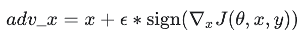
: Our output adversarial image
  • x: The original input image
  • y: The ground-truth label of the input image
  • \epsilon: Small value we multiply the signed gradients by to ensure the perturbations are small enough that the human eye cannot detect them but large enough that they fool the neural network
  • \theta: Our neural network model
  • J: The loss function

If you’re struggling to follow the math surrounding FGSM, don’t worry, it will be much easier to understand once we start looking at some code later in this guide.

Configuring your development environment

This tutorial on adversarial images with FGSM utilizes Keras and TensorFlow. If you intend to follow this tutorial, I suggest you take the time to configure your deep learning development environment.

You can utilize either of these two guides to install TensorFlow and Keras on your system:

Either tutorial will help configure your system with all the necessary software for this blog post in a convenient Python virtual environment.

Having problems configuring your development environment?

Figure 3: Having trouble configuring your dev environment? Want access to pre-configured Jupyter Notebooks running on Google Colab? Be sure to join PyImageSearch Plus — you’ll be up and running with this tutorial in a matter of minutes.

All that said, are you:

  • Short on time?
  • Learning on your employer’s administratively locked system?
  • Wanting to skip the hassle of fighting with the command line, package managers, and virtual environments?
  • Ready to run the code right now on your Windows, macOS, or Linux systems?

Then join PyImageSearch Plus today!

Gain access to Jupyter Notebooks for this tutorial and other PyImageSearch guides that are pre-configured to run on Google Colab’s ecosystem right in your web browser! No installation required.

And best of all, these Jupyter Notebooks will run on Windows, macOS, and Linux!

Project structure

Let’s get started by reviewing our project directory structure. Be sure to access the “Downloads” section of this tutorial to retrieve the source code:

$ tree . --dirsfirst
.
├── pyimagesearch
│   ├── __init__.py
│   ├── fgsm.py
│   └── simplecnn.py
└── fgsm_adversarial.py

1 directory, 4 files

Inside the pyimagesearch module, we have two Python scripts we’ll be implementing:

  1. simplecnn.py: A basic CNN architecture
  2. fgsm.py: Our implementation of the Fast Gradient Sign Method adversarial attack

The fgsm_adversarial.py file is our driver script. It will:

  1. Instantiate an instance of SimpleCNN
  2. Train it on the MNIST dataset
  3. Demonstrate how to apply the FGSM adversarial attack to the trained model

Creating a simple CNN architecture for adversarial training

Before we can perform an adversarial attack, we first need to implement our CNN architecture.

Once our architecture is implemented, we’ll train it on the MNIST dataset, evaluate it, generate a set of adversarial images using the FGSM, and re-evaluate it, thereby demonstrating the impact adversarial images have on accuracy.

In next week and the following week’s tutorials, you’ll learn training techniques that you can use to defend against these adversarial attacks.

But it all starts with implementing the CNN architecture — open the simplecnn.py in the pyimagesearch module of our project directory structure and let’s get to work:

# import the necessary packages
from tensorflow.keras.models import Sequential
from tensorflow.keras.layers import BatchNormalization
from tensorflow.keras.layers import Conv2D
from tensorflow.keras.layers import Activation
from tensorflow.keras.layers import Flatten
from tensorflow.keras.layers import Dropout
from tensorflow.keras.layers import Dense

We start on Lines 2-8, importing our required Keras/TensorFlow classes. These are all fairly standard imports when training a CNN.

If you’re new to Keras and TensorFlow, I suggest you read my introductory Keras tutorial along with my book, Deep Learning for Computer Vision with Python, which covers deep learning in detail.

With our imports taken care of, we can define our CNN architecture:

class SimpleCNN:
	@staticmethod
	def build(width, height, depth, classes):
		# initialize the model along with the input shape
		model = Sequential()
		inputShape = (height, width, depth)
		chanDim = -1

		# first CONV => RELU => BN layer set
		model.add(Conv2D(32, (3, 3), strides=(2, 2), padding="same",
			input_shape=inputShape))
		model.add(Activation("relu"))
		model.add(BatchNormalization(axis=chanDim))

		# second CONV => RELU => BN layer set
		model.add(Conv2D(64, (3, 3), strides=(2, 2), padding="same"))
		model.add(Activation("relu"))
		model.add(BatchNormalization(axis=chanDim))

		# first (and only) set of FC => RELU layers
		model.add(Flatten())
		model.add(Dense(128))
		model.add(Activation("relu"))
		model.add(BatchNormalization())
		model.add(Dropout(0.5))

		# softmax classifier
		model.add(Dense(classes))
		model.add(Activation("softmax"))

		# return the constructed network architecture
		return model

The build method of our SimpleCNN class accepts four parameters:

  1. width: Width of the input images in our dataset
  2. height: Height of the input images in our dataset
  3. channels: Number of channels in the images
  4. classes: Total number of unique classes in the dataset

From there, we define a Sequential network consisting of:

  1. A first set of CONV => RELU => BN layers. The CONV layer learns a total of 32 3×3 filters with 2×2 strided convolution to reduce volume size.
  2. A second set of CONV => RELU => BN layers. Same as above, but this time the CONV layer learns 64 filters.
  3. A set of dense/fully-connected layers. The output of which is our softmax classifier used for returning probabilities for each class label.

Now that our architecture has been implemented, we can move on to the Fast Gradient Sign Method.

Implementing the Fast Gradient Sign Method with Keras and TensorFlow

The adversarial attack method we will implement is called the Fast Gradient Sign Method (FGSM). It’s called this method because:

  1. It’s fast (it’s in the name)
  2. We construct the image adversary by calculating the gradients of the loss, computing the sign of the gradient, and then using the sign to build the image adversary

Let’s implement the FGSM now. Open the fgsm.py file in your project directory structure and insert the following code:

# import the necessary packages
from tensorflow.keras.losses import MSE
import tensorflow as tf

def generate_image_adversary(model, image, label, eps=2 / 255.0):
	# cast the image
	image = tf.cast(image, tf.float32)

Lines 2 and 3 import our required Python packages. We’ll be using the mean-squared error (MSE) loss function for computing our adversarial attack, but you could also use any other appropriate loss function for the task, including categorical cross-entropy, binary cross-entropy, etc.

Line 5 starts the definition of our FGSM attack, generate_image_adversary. This function accepts four parameters:

  1. The model that we are trying to fool
  2. The input image that we want to misclassify
  3. The ground-truth class label of the input image
  4. A small eps value that weights the gradient update — a small-ish value should be used here such that the gradient update is large enough to cause the input image to be misclassified but not so large that the human eye can tell the image has been manipulated

Let’s start implementing the FGSM attack now:

	# record our gradients
	with tf.GradientTape() as tape:
		# explicitly indicate that our image should be tacked for
		# gradient updates
		tape.watch(image)

		# use our model to make predictions on the input image and
		# then compute the loss
		pred = model(image)
		loss = MSE(label, pred)

Line 10 instructs TensorFlow to record our gradients, while Line 13 explicitly tells TensorFlow that we want to track the gradient updates on our input image.

From there, we use our model to make predictions on the image and then compute our loss using mean-squared error (again, you can substitute another loss function here for your task, but MSE is a fairly standard choice).

Next, let’s implement the “signed gradient” portion of the FGSM attack:

	# calculate the gradients of loss with respect to the image, then
	# compute the sign of the gradient
	gradient = tape.gradient(loss, image)
	signedGrad = tf.sign(gradient)

	# construct the image adversary
	adversary = (image + (signedGrad * eps)).numpy()

	# return the image adversary to the calling function
	return adversary

Line 22 computes the gradients of the loss with respect to the image.

We then take the sign of the gradient on Line 23 (hence the term, Fast Gradient Sign Method). The output of this line of code is a vector filled with three values — either 1 (positive), 0, or -1 (negative).

Using this information, Line 26 creates our image adversary by:

  1. Taking the signed gradient and multiplying it by a small epsilon factor. The goal here is to make our gradient update large enough to misclassify the input image but not so large that the human eye can tell the image has been tampered.
  2. We then add this small delta value to our image, which ever so slightly changes the pixel intensity values in the image.

These pixel updates will be undetectable to the human eye, but according to our CNN, the image will appear vastly different, resulting in misclassification.

Creating our adversarial training script

With both our CNN architecture and FGSM implemented, we can move on to creating our training script.

Open the fgsm_adversarial.py script in our directory structure, and we can get to work:

# import the necessary packages
from pyimagesearch.simplecnn import SimpleCNN
from pyimagesearch.fgsm import generate_image_adversary
from tensorflow.keras.optimizers import Adam
from tensorflow.keras.utils import to_categorical
from tensorflow.keras.datasets import mnist
import numpy as np
import cv2

Lines 2-8 import our required Python packages. Our notable imports include SimpleCNN (our basic CNN architecture we implemented earlier in this guide) and generate_image_adversary (our helper function to perform the FGSM attack).

We’ll be training our SimpleCNN architecture on the mnist dataset. The model will be trained with categorical cross-entropy loss and the Adam optimizer.

With the imports taken care of, we can now load the MNIST dataset from disk:

# load MNIST dataset and scale the pixel values to the range [0, 1]
print("[INFO] loading MNIST dataset...")
(trainX, trainY), (testX, testY) = mnist.load_data()
trainX = trainX / 255.0
testX = testX / 255.0

# add a channel dimension to the images
trainX = np.expand_dims(trainX, axis=-1)
testX = np.expand_dims(testX, axis=-1)

# one-hot encode our labels
trainY = to_categorical(trainY, 10)
testY = to_categorical(testY, 10)

Line 12 loads the pre-split MNIST dataset from disk. We preprocess the MNIST dataset by:

  1. Scaling the pixel intensities from the range [0, 255] to [0, 1]
  2. Adding a batch dimension to the images
  3. One-hot encoding the labels

From there, we can initialize our SimpleCNN model:

# initialize our optimizer and model
print("[INFO] compiling model...")
opt = Adam(lr=1e-3)
model = SimpleCNN.build(width=28, height=28, depth=1, classes=10)
model.compile(loss="categorical_crossentropy", optimizer=opt,
	metrics=["accuracy"])

# train the simple CNN on MNIST
print("[INFO] training network...")
model.fit(trainX, trainY,
	validation_data=(testX, testY),
	batch_size=64,
	epochs=10,
	verbose=1)

# make predictions on the testing set for the model trained on
# non-adversarial images
(loss, acc) = model.evaluate(x=testX, y=testY, verbose=0)
print("[INFO] loss: {:.4f}, acc: {:.4f}".format(loss, acc))

Lines 26-29 initializes our CNN. We then train it on Lines 33-37.

Evaluation occurs on Lines 41 and 42, displaying our loss and accuracy computed over the test set. We show this information to demonstrate that our CNN is doing a good job at making predictions on the testing set…

…that is until it’s time to generate adversarial images. That’s when we’ll see our accuracy fall apart.

Speaking of which, let’s generate some adversarial images using the FGSM now:

# loop over a sample of our testing images
for i in np.random.choice(np.arange(0, len(testX)), size=(10,)):
	# grab the current image and label
	image = testX[i]
	label = testY[i]

	# generate an image adversary for the current image and make
	# a prediction on the adversary
	adversary = generate_image_adversary(model,
		image.reshape(1, 28, 28, 1), label, eps=0.1)
	pred = model.predict(adversary)

On Line 45, we loop over a sample of ten randomly selected testing images. Lines 47 and 48 grab the image and ground-truth label for the current image.

From there, we can use our generate_image_adversary function to create the image adversary using the Fast Gradient Sign Method (Lines 52 and 53).

Specifically, take note of the image.reshape call where we are ensuring the image has a shape of (1, 28, 28, 1). These values are:

  • 1: Batch dimension; we’re working with a single image here, so the value is trivially set to one.
  • 28: Height of the image
  • 28: Width of the image
  • 1: Number of channels in the image (MNIST images are grayscale, hence only one channel)

With our image adversary generated, we ask our model to make predictions on it via Line 54.

Let’s now prepare the image and adversary for visualization:

	# scale both the original image and adversary to the range
	# [0, 255] and convert them to an unsigned 8-bit integers
	adversary = adversary.reshape((28, 28)) * 255
	adversary = np.clip(adversary, 0, 255).astype("uint8")
	image = image.reshape((28, 28)) * 255
	image = image.astype("uint8")

	# convert the image and adversarial image from grayscale to three
	# channel (so we can draw on them)
	image = np.dstack([image] * 3)
	adversary = np.dstack([adversary] * 3)

	# resize the images so we can better visualize them
	image = cv2.resize(image, (96, 96))
	adversary = cv2.resize(adversary, (96, 96))

Keep in mind that our preprocessing steps included scaling our training/testing images from the range [0, 255] to [0, 1]to visualize our images with OpenCV, we now need to undo these preprocessing operations.

Lines 58-61 scale our image and adversary, ensuring they are both unsigned 8-bit integer data types.

We’d like to draw the predictions for both the original image and adversarial image in either green (correct) or red (incorrect). To do that, we must convert our images from grayscale to an RGB representation of a grayscale image (Lines 65 and 66).

MNIST images are only 28×28, which can be hard to see, especially on a high-resolution screen, so we increase the image sizes to 96×96 on Lines 69 and 70.

Our final code block rounds out the visualization process:

	# determine the predicted label for both the original image and
	# adversarial image
	imagePred = label.argmax()
	adversaryPred = pred[0].argmax()
	color = (0, 255, 0)

	# if the image prediction does not match the adversarial
	# prediction then update the color
	if imagePred != adversaryPred:
		color = (0, 0, 255)

	# draw the predictions on the respective output images
	cv2.putText(image, str(imagePred), (2, 25),
		cv2.FONT_HERSHEY_SIMPLEX, 0.95, (0, 255, 0), 2)
	cv2.putText(adversary, str(adversaryPred), (2, 25),
		cv2.FONT_HERSHEY_SIMPLEX, 0.95, color, 2)

	# stack the two images horizontally and then show the original
	# image and adversarial image
	output = np.hstack([image, adversary])
	cv2.imshow("FGSM Adversarial Images", output)
	cv2.waitKey(0)

Lines 74 and 75 grab the MNIST digit predictions.

We initialize the color of our labels to be “green” (Line 76) if both the imagePred and adversaryPred are equal. This will happen if our model can correctly label the adversarial image. Otherwise, we’ll update our prediction color to be red (Lines 80 and 81).

We then draw the imagePred and adversaryPred on their respective images (Lines 84-87).

The final step is to visualize both the image and adversary next to each other so we can see if our adversarial attack was successful or not.

FGSM training results

We are now ready to see the Fast Gradient Sign Method in action!

Start by accessing the “Downloads” section of this tutorial to retrieve the source code. From there, open a terminal and execute the fgsm_adversarial.py script:

$ python fgsm_adversarial.py
[INFO] loading MNIST dataset...
[INFO] compiling model...
[INFO] training network...
Epoch 1/10
938/938 [==============================] - 12s 13ms/step - loss: 0.1945 - accuracy: 0.9407 - val_loss: 0.0574 - val_accuracy: 0.9810
Epoch 2/10
938/938 [==============================] - 12s 13ms/step - loss: 0.0782 - accuracy: 0.9761 - val_loss: 0.0584 - val_accuracy: 0.9814
Epoch 3/10
938/938 [==============================] - 13s 13ms/step - loss: 0.0594 - accuracy: 0.9817 - val_loss: 0.0624 - val_accuracy: 0.9808
Epoch 4/10
938/938 [==============================] - 13s 14ms/step - loss: 0.0479 - accuracy: 0.9852 - val_loss: 0.0411 - val_accuracy: 0.9867
Epoch 5/10
938/938 [==============================] - 12s 13ms/step - loss: 0.0403 - accuracy: 0.9870 - val_loss: 0.0357 - val_accuracy: 0.9875
Epoch 6/10
938/938 [==============================] - 12s 13ms/step - loss: 0.0365 - accuracy: 0.9884 - val_loss: 0.0405 - val_accuracy: 0.9863
Epoch 7/10
938/938 [==============================] - 12s 13ms/step - loss: 0.0310 - accuracy: 0.9898 - val_loss: 0.0341 - val_accuracy: 0.9889
Epoch 8/10
938/938 [==============================] - 12s 13ms/step - loss: 0.0289 - accuracy: 0.9905 - val_loss: 0.0388 - val_accuracy: 0.9873
Epoch 9/10
938/938 [==============================] - 12s 13ms/step - loss: 0.0217 - accuracy: 0.9928 - val_loss: 0.0652 - val_accuracy: 0.9811
Epoch 10/10
938/938 [==============================] - 11s 12ms/step - loss: 0.0216 - accuracy: 0.9925 - val_loss: 0.0396 - val_accuracy: 0.9877
[INFO] loss: 0.0396, acc: 0.9877

As you can see, our script has obtained 99.25% accuracy on our training set and 98.77% accuracy on the testing set, implying that our model is doing a good job at making digit predictions.

However, let’s see what happens when we generate adversarial images using FGSM:

Figure 4: The results of applying adversarial image training using the FGSM. Example digits are shown before FGSM adversarial attack (green) followed by after (red). These pairs of digits are essentially identical to the human eye, but according to our CNN, are misclassified.

Figure 4 displays a montage of ten images, including the original MNIST image from the testing set (left) and the output FGSM image (right).

Visually, the adversarial FGSM images are identical to the original digit images; however, our CNN is completely fooled, making incorrect predictions for each of the images.

What’s the big deal?

Fooling a CNN using adversarial images and causing it to make incorrect predictions on the MNIST dataset seems low consequence.

But what happens if that model were trained to detect pedestrians crossing the street and deployed to a self-driving car? There would be tremendous consequences as now people’s lives would be on the line.

That raises the question:

If it’s so easy to fool CNNs, what can we do to defend against adversarial attacks?

In the next two blog posts, I’ll show you how to defend against adversarial attacks by updating our training procedure to include adversarial images.

Credits and references

The FGSM implementation was inspired by Sebastian Theiler’s excellent article on adversarial attacks and defenses. A huge shoutout and thank you to Sebastian for sharing his knowledge.

What’s next?

Figure 5: Join PyImageSearch University and learn Computer Vision using OpenCV and Python. Enjoy guided lessons, quizzes, assessments, and certifications. You’ll learn everything from deep learning foundations applied to computer vision up to advanced, real-time augmented reality. Don’t worry; it will be fun and easy to follow because I’m your instructor. Won’t you join me today to further your computer vision and deep learning study?

Would you enjoy learning how to successfully and confidently apply OpenCV to your projects?

Are you worried that configuring your development environment for Computer Vision, Deep Learning, and OpenCV will be too challenging, resulting in confusing, hard to debug error messages?

Concerned that you’ll get lost sifting through endless tutorials and video guides as you struggle to master Computer Vision?

No problem, because I’ve got you covered. PyImageSearch University is your chance to learn from me at your own pace.

You’ll find everything you need to master the basics (like we did together in this tutorial) and move on to advanced concepts.

Don’t worry about your operating system or development environment. I’ve got you covered with pre-configured Jupyter Notebooks in Google Colab for every tutorial on PyImageSearch, including Jupyter Notebooks for our new weekly tutorials as well!

Best of all, these Jupyter Notebooks will run on your machine, regardless of whether you are using Windows, macOS, or Linux! Irrespective of the operating system used, you will still be able to follow along and run the code in every lesson (all inside the convenience of your web browser).

Additionally, you can massively accelerate your progress by watching our video lessons accompanying each post. Every lesson at PyImageSearch University includes a detailed, step-by-step video guide.

You may feel that learning Computer Vision, Deep Learning, and OpenCV is too hard. Don’t worry; I’ll guide you gradually through each lecture and topic, so we build a solid foundation, and you grasp all the content.

When you think about it, PyImageSearch University is almost an unfair advantage compared to self-guided learning. You’ll learn more efficiently and master Computer Vision faster.

Oh, and did I mention you’ll also receive Certificates of Completion as you progress through each course at PyImageSearch University?

I’m sure PyImageSearch University will help you master OpenCV drawing and all the other computer vision skills you will need. Why not join today?

Summary

In this tutorial, you learned how to implement the Fast Gradient Sign Method (FGSM) for adversarial image generation. We implemented FGSM using Keras and TensorFlow, but you can certainly translate the code into a deep learning library of your choosing.

The FGSM works by:

  1. Taking an input image
  2. Making predictions on the image using a trained CNN
  3. Computing the loss of the prediction based on the true class label
  4. Calculating the gradients of the loss with respect to the input image
  5. Computing the sign of the gradient
  6. Using the signed gradient to construct the output adversarial image

It may sound complicated, but as we saw, we were able to implement FGSM in under 30 lines of code, thanks to TensorFlow’s fantastic GradientTape function, which makes gradient computation a breeze.

Now that you learned how to construct adversarial images using FGSM, you’ll learn how to defend against these attacks by incorporating adversarial images into your training process next week.

Stay tuned. You won’t want to miss this tutorial!

To download the source code to this post (and be notified when future tutorials are published here on PyImageSearch), simply enter your email address in the form below!

Download the Source Code and FREE 17-page Resource Guide

Enter your email address below to get a .zip of the code and a FREE 17-page Resource Guide on Computer Vision, OpenCV, and Deep Learning. Inside you'll find my hand-picked tutorials, books, courses, and libraries to help you master CV and DL!

The post Adversarial attacks with FGSM (Fast Gradient Sign Method) appeared first on PyImageSearch.

An interview with Anthony Lowhur – Recognizing 10,000 Yugioh Cards with Computer Vision and Deep Learning

$
0
0

In this blog post, I interview computer vision and deep learning engineer, Anthony Lowhur. Anthony shares the algorithms and techniques that he used to build a computer vision and deep learning system capable of recognizing 10,000+ Yugioh trading cards.

I love Anthony’s project — and I wish I had it years ago.

When I was a kid, I loved to collect trading cards. I had binders and binders filled with baseball cards, basketball cards, football cards, Pokemon cards, etc. I even had Jurassic Park trading cards!

I cannot even begin to estimate the number of hours I spent organizing my cards, grouping them first by team, then by position, and finally in alphabetical order.

Then, when I was done, I would come up with a “new and better way” to sort the cards and start all over again. At a young age, I was exploring the algorithmic complexity where an eight-year-old can sort cards. At best, I was probably only O(N2), so I had quite a bit of room for improvement.

Anthony has taken card recognition to an entirely new level. Using your smartphone, you can snap a photo of a Yugioh trading card and instantly recognize it. Such an application is useful for:

  • Collectors who want to quickly determine if a trading card is already in their collection
  • Archivists who want to build databases of Yugioh cards, their attributes, hit points, damage, etc. (i.e., OCR the card after recognition)
  • Yugioh players who want not only to recognize a card but also translate it as well (very useful if you cannot read Japanese but want to play with both English and Japanese cards at the same time, or vice versa).

Anthony built his Yugioh card recognition system using several computer vision and deep learning algorithms, including:

  • Siamese networks
  • Triplet loss
  • Keypoint matching for final reranking (this is an especially clever trick that you’ll want to learn more about)

Join me as I sit down with Anthony and discuss his project.

To learn how to recognize Yugioh cards with computer vision and deep learning, just keep reading.

An interview with Anthony Lowhur – Recognizing 10,000 Yugioh Cards with Computer Vision and Deep Learning

Adrian: Welcome, Anthony! Thank you so much for being here. It’s a pleasure to have you on the PyImageSearch blog.

Anthony: Thank you for having me. It’s an honor to be here.


Adrian: Tell us a bit about yourself — where do you work and what is your job?

Anthony: I am currently a full-time computer vision (CV) and machine learning (ML) engineer not far from Washington DC, and I design and build Artificial Intelligence (AI) systems that would be used by clients. I actually graduated and got my bachelor’s from the university not too long ago, so I am still quite fresh in the industry.


Adrian: How did you first become interested in computer vision and deep learning?

Anthony: I was a high school student when I started to learn about a self-driving car competition known as the DARPA Grand Challenge. It is essentially a competition among different universities and research labs to build autonomous vehicles to race against each other in the desert. The car that won the competition was from Stanford University, lead by Sebastian Thrun.

Sebastian Thrun then went on to lead the Google X project in creating a self-driving car. The fact that something previously considered part of science fiction is now becoming a reality really inspired me, and I began learning about computer vision and deep learning after that. I began to do personal projects in CV and ML and began to conduct CV/ML research at REUs (Research Experiences for Undergraduates), and everything took off from there.


Adrian: You just finished developing a computer vision system that can automatically recognize 10,000+ Yugioh cards. Fantastic job! What inspired you to create such a system? And how can such a system help Yugioh players and card collectors?

Anthony: So there is a card game and TV series known as Yugioh that I watched when I was a child. It was something that held my heart to this day, and it brings out the nostalgia of sitting in front of the TV after returning from school each day.

Figure 1: A Yugioh duel disk.

I added the AI because making it was actually a prerequisite to an even bigger project, which was a Yugioh duel disk.

You can read more information about it here: I made a functional Duel Disk (powered by AI).

And here is a demo video:

In a nutshell, it’s a flashy device that allows you to duel each other a few feet away, which made its appearance in the TV series. I thought of this as a fun project to make and show to other Yugioh fans, which was enough to motivate me and continue the project until its prototype completion.

Other than for creating the duel disk, I have had people come to me saying that they were interested in having it either organize their Yugioh card collection or to power one of their app ideas. Though there are some imperfections, it is currently open-sourced on GitHub, so people have the chance to try it out.


Adrian: How did you build your dataset of Yugioh cards? And how many example images per card did you end up with?

Anthony: First, I had to extract our dataset. The card dataset was retrieved from an API. The full-size version of the cards was used: Yu-Gi-Oh! API Guide – YGOPRODECK.

The API was used to download all Yugioh cards (10,856 cards) onto our machine to turn them into a dataset.

However, the main problem is that most cards only contain one card art (and other cards with multiple card arts have card arts that are significantly different from each other). In a machine learning sense, essentially, there are over 10,000 classes where each of those classes contains only one image each.

This is a problem, as traditional deep learning methods would not do well on datasets with lower than a hundred images, let alone one image per class. And I was doing this for 10,000 classes.

As a result, I would have to use one-shot learning to tackle this problem. One-shot learning is a method that compares the similarity between two images rather than predicts a class.

Figure 2: Anthony used data augmentation to generate multiple versions of each Yugioh card.

Adrian: With essentially only one example image per card, you don’t have much to learn from a neural network. Did you apply any type of data augmentation? If so, what type of data augmentation did you use?

Anthony: While we are working with only one image per class, we want to see if we can get as much robustness from this model as we possibly can. As a result, we perform image augmentation to create multiple versions of each card art, but with subtle differences (brightness change, contrast change, shifting, etc.). This will give our network slightly more data to work with, allowing our model to generalize better.


Adrian: You now have a dataset of Yugioh cards on your disk. How did you go about choosing a deep learning model architecture?

Anthony: So originally, I experimented with a simple shallow network for the siamese network as a sort of benchmark to measure.

Not surprisingly, the network did not perform that well. The network was underfitting the training data I was giving it, so I thought about resolving that. Adding more layers to the network is one of the remedies to the solution, so I tried out Resnet101, a network widely known for its massive layer depth. That ended up being the architecture I needed as it performed significantly better and was obtaining my accuracy goal. Consequently, this has been the resulting main architecture.

Of course, if I later desire to make the inference time of a single image prediction faster, I could always resort to using a network with fewer layers like VGG16, though.


Adrian: You clearly did your homework here and knew that siamese networks were the best architecture choice for this project. Did you use standard “vanilla” siamese networks with image pairs? Or did you use triplets and triplet loss to train your network?

Anthony: Originally, I tried vanilla siamese networks that mainly used a pair of images to make comparisons, though its limitations started to show.

As a result, I researched other architectures, and I eventually discovered the triplet net. It mainly differs from siamese networks as it uses three images instead of two and uses a different loss function known as triplet loss. It was mainly able to manipulate distances between images using positive and negative anchors during the training process. Consequently, it was relatively quick to implement and just happen to be the resulting solution.


Adrian: At this point, you have a deep learning model that can either identify an input Yugioh card or be very close to returning the correct Yugioh card in the top-10 results. How did you improve accuracy further? Did you employ some sort of image re-ranking algorithm?

Anthony: So while triplet net made from resnet101 showed significant improvement, there seems to be some borderline cases in which it doesn’t predict the correct rank-1 class but came relatively close. To overcome this, the ORB (Oriented FAST and Rotated BRIEF) algorithm is used as support. ORB is an algorithm that searches for feature points within an image, so if two images are completely identical, the two images should have the same amount of feature points as each other.

This algorithm serves as a support to our one-shot learning method. As soon as our neural network generates a score on all 10,000 cards and ranks them, our ORB takes the top-N card ranking (e.g., top 50 cards) and calculates the number of ORB points on the images. The original similarity score and number of ORB points are then fed into a formula to obtain a final weighted similarity score. The weighted score of the top-N cards is compared, and the scores are rearranged to their final rankings.

Figure 3: Using key points to re-rank the top-N results from the siamese network. This re-ranking improves Yugioh card recognition accuracy.

Figure 3 shows a previously challenging edge case in which we compare two images of the top card (Dark Magician) in different contrast settings. Originally failed without ORB matching support, but considering the number of feature points in mind, we can get a more accurate ranking.

After some experimentation and tuning of certain values, I improved the number of correct predictions significantly.


Adrian: During your experimentation, you found that even small shifts/translations in your input images could cause significant drops in accuracy, implying that your Convolutional Neural Network (CNN) wasn’t handling translation well. How did you overcome this problem?

Anthony: It was indeed interesting and tricky to deal with this problem. Modern CNNs are in nature not shift-invariant, and that even small translations can confuse it. This is further emphasized by the fact we are dealing with very little data and that the algorithm was reliant on comparing feature maps together to make predictions.

Figure 4: Slight translations caused drops in Yugioh card recognition accuracy.
  • On the left side, the original image is compared with the same image but translated to the right (we jumped up by 0.71 points).
  • In the middle image, the original image is compared with the same image but translated to the right and upward.
  • In the right image, the original image is compared with the same image but translated to the right and upward.

This problem shows that our model would be very sensitive to slight misalignment and prevent our model from achieving its full potential.

My first approach was to simply augment the data by adding more translations in the data augmentation process. However, this was not enough, and I had to look into other methods.

As a result, I found some research that created the blur pooling algorithm for tackling a similar problem. Blur pooling is a method made to solve the problem of CNNs not being sift-invariant and applied at the end of every convolution layer.


Adrian: Your algorithm works by essentially generating a similarity score for all cards in your dataset. Did you encounter any speed or efficiency issues from comparing an input Yugioh card among 10,000+ cards?

Anthony: So, at this point, I have a model capable of generating similarity scores of every card at a reasonable accuracy. Now all I have to do is generate similarity scores for our input image and all the cards I wish to compare.

If I measure my model’s inference time, we can see that it takes around 0.12 seconds to pass a single image through our Triplet Resnet architecture along with an 0.08-second image preprocessing step. This does not sound bad on the surface, but remember that we have to do this on all cards we have in the dataset. The problem is that there are over 10,000 cards we will have to compare with the input and generate its score.

So if we take the number of seconds it takes to generate a similarity score and the total amount of cards (10,856) there are in the dataset, we get this:

(0.12+0.08) * 10,856 = 2171.2 s

2171.2/60 = 36.2 minutes

To predict what a single input image is, we would have to wait well over 30 minutes. This does not make our model practical to use as a result.

Figure 5: Example of a dictionary data structure.

To solve this, I ended up pre-calculating the output convolutional feature maps of all 10,000 cards ahead of time and storing them in a dictionary. The great thing about dictionaries is that retrieving the pre-calculated feature maps from them would be constant time (O(1) time). So this would do a decent job scaling with the number of cards in the dataset.

So what happens is that after training, we iterate through over 10,000 cards, feed them into our triplet net to get the output convolution feature map, and store that in our dictionary. We just iterate through our new dictionary in the prediction phase instead of having our model performing forward propagation 10,000 times.

Figure 6: Final inference time measurement ran on Jetson Nano. It takes around 5 seconds to generate a prediction on an embedded device.

As a result, the previous single-image prediction time of 36 minutes has been significantly reduced by close to 5 seconds. This results in a more manageable model.


Adrian: How did you test and evaluate the accuracy of your Yugioh card recognition system?

Anthony: So overall, I was dealing with essentially two types of datasets.

I used a dataset for training, where official card art images were used from the ygoprodeck (dataset A) along with real-life photos of cards in the wild (dataset B), which were pictures of cards taken by a camera. Dataset B is essentially the ultimate testing dataset I used to succeed in the long run.

The AI/machine learning model was tested on real photos of cards (cards with and without sleeves). This is an example of dataset B.

Figure 7: Left card has a card sleeve, the right one is without.

These types of images are what I ultimately want my AI classifier to be successful in having a camera point down at your card and be able to recognize it.

However, since buying over 10,000 cards and taking pictures of them wasn’t a realistic scenario, I tried the next best thing: to test it on an online dataset of Yugioh cards and artificially add challenging modifications. Modifications included changing brightness, contrast, and shear to simulate Yugioh cards under different lighting/photo quality scenarios in real life (dataset A).

Here are some of the input images and the card art from the dataset:

Figure 8: Batch of images under different contrast/lighting conditions. Left of each pair is the input image, right is the card art from the dataset.

And these are the final results:

Figure 9: Obtaining \approx
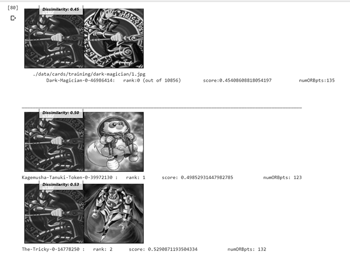
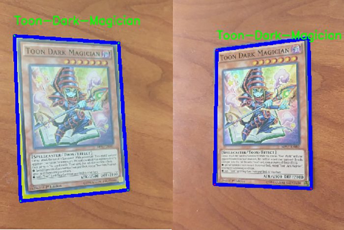
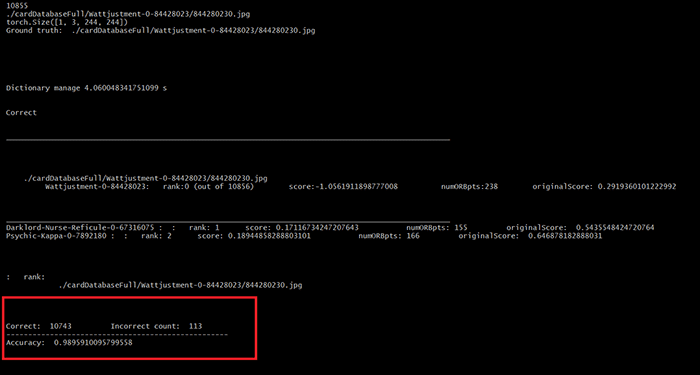
99% accuracy with Yugioh card recognition.

Here are a few examples of the card recognizer in action:

Figure 10: Model can handle differences in orientation, angle shots, and blurs to an extent.

The AI classifier managed to achieve around 99% accuracy on all the cards in the game of Yugioh.

This was meant to be a quick project, so I am happy with the progress. I may try to see if I can gather more Yugioh cards and try to improve the system.


Adrian: What are the next steps for your project?

Anthony: There are definitely some imperfections that prevent my model from reaching its full potential.

The dataset used for training were official card art images from the ygoprodeck (dataset A) and not real-life photos of cards in the wild (dataset B), which are pictures of cards taken by a camera.

The 99% accuracy results were from training and testing on dataset A while the trained model was also tested on a handful of cards on dataset B. However, we don’t have a lot of data for dataset B to perform actual training on it or even mass-evaluation. This repo proves that our model can learn Yugioh cards through dataset A and has the potential to succeed with dataset B, which is the more realistic and natural set of images goal for our model. Setting up a data collection infrastructure to mass-collect image samples for dataset B would significantly advance this project and help confirm the model’s strength.

This program also does not have a proper object detector and just uses simple image processing methods (4 point transformation) to get the card’s bounding box and align it. Using a proper object detector like YOLO (you only look once) would be ideal, which would also help detect multiple demo cards.

More accurate and realistic image augmentation methods would help add glares, more natural lighting, and warps, which may help my model adapt from dataset A to even more real-life images.


Adrian: You’ve been a PyImageSearch reader and customer since 2017! Thank you for supporting PyImageSearch and me. What PyImageSearch books and courses do you own? And how did they help prepare you for this project’s completion?

Anthony: I currently own the Deep Learning for Computer Vision for Python bundle as well as the Raspberry Pi for Computer Vision book.

The time gap between reading your books and my attempt at this project is around 3 years, so there have been many things I have experienced and picked up from various sources along the way.

The PyImageSearch blog and Deep Learning for Computer Vision with Python bundle have been part of my immense journey, teaching me and strengthening my computer vision and deep learning fundamentals. Thanks to the bundle, I became aware of more architectures like Resnet and methods like transfer learning. They have helped form my base knowledge to dive into more advanced concepts that I would not have normally experienced.

By the time I started to tackle the Yugioh project, most of the concepts that I had applied in the project were second nature to me. They gave me the confidence to plan out and experiment with models until I received satisfying results.


Adrian: Would you recommend these books and courses to other budding developers, students, and researchers trying to learn computer vision, deep learning, and OpenCV?

Anthony: Certainly, books such as Deep Learning for Computer Vision with Python have a wealth of knowledge that can be used to jumpstart or strengthen anyone’s computer vision and machine learning journey. Its explanations for each topic, along with code examples, make it easy to follow along with giving a wide breadth of information. It has definitely strengthened my fundamentals in the field and helped me transition into being able to pick up even more advanced topics that I would not have learned otherwise.


Adrian: If a PyImageSearch reader wants to chat about your project, what is the best place to connect with you?

Anthony: The best way to contact me is through my email at antlowhur [at] yahoo [dot] com

You can also reach me on LinkedIn, Medium, and if you want to see more of my projects, check out my GitHub page.

Summary

Today we interviewed Anthony Lowhur, computer vision and deep learning engineer.

Anthony created a computer vision project capable of recognizing over 10,000 Yugioh trading cards.

His algorithm worked by:

  1. Using data augmentation to generate additional data samples for each Yugioh card
  2. Training a siamese network on the data
  3. Pre-computing feature maps and distances between cards (useful to achieve faster card recognition)
  4. Utilizing keypoint matching to rerank the top outputs from the siamese network model

Overall, his system was nearly 99% accurate!

To be notified when future tutorials and interviews are published here on PyImageSearch, simply enter your email address in the form below!

Download the Source Code and FREE 17-page Resource Guide

Enter your email address below to get a .zip of the code and a FREE 17-page Resource Guide on Computer Vision, OpenCV, and Deep Learning. Inside you'll find my hand-picked tutorials, books, courses, and libraries to help you master CV and DL!

The post An interview with Anthony Lowhur – Recognizing 10,000 Yugioh Cards with Computer Vision and Deep Learning appeared first on PyImageSearch.

Defending against adversarial image attacks with Keras and TensorFlow

$
0
0

In this tutorial, you will learn how to defend against adversarial image attacks using Keras and TensorFlow.

So far, you have learned how to generate adversarial images using three different methods:

  1. Adversarial images and attacks with Keras and TensorFlow
  2. Targeted adversarial attacks with Keras and TensorFlow
  3. Adversarial attacks with FGSM (Fast Gradient Sign Method)

Using adversarial images, we can trick our Convolutional Neural Networks (CNNs) into making incorrect predictions. While, according to the human eye, adversarial images may look identical to their original counterparts, they contain small perturbations that cause our CNNs to make wildly incorrect predictions.

As I discuss in this tutorial, there are enormous consequences to deploying undefended models into the wild.

For example, imagine a deep neural network deployed to a self-driving car. Nefarious users could generate adversarial images, print them, and then apply them to the road, signs, overpasses, etc., which would result in the model thinking there were pedestrians, cars, or obstacles when there are, in fact, none! The result could be disastrous, including car accidents, injuries, and loss of life.

Given the risk that adversarial images pose, that raises the question:

What can we do to defend against these attacks?

We’ll be addressing that question in a two-part series on adversarial image defense:

  1. Defending against adversarial image attacks with Keras and TensorFlow (today’s tutorial)
  2. Mixing normal images and adversarial images when training CNNs (next week’s guide)

Adversarial image defense is no joke. If you’re deploying models into the real-world, then be sure you have procedures in place to defend against adversarial attacks.

By following these tutorials, you can train your CNNs to make correct predictions even if they are presented with adversarial images.

To learn how to train a CNN to defend against adversarial attacks with Keras and TensorFlow, just keep reading.

Looking for the source code to this post?

Jump Right To The Downloads Section

Defending against adversarial image attacks with Keras and TensorFlow

In the first part of this tutorial, we’ll discuss the concept of adversarial images as an “arms race” and what we can do to defend against them.

We’ll then discuss two methods that we can use to defend against adversarial images. We’ll implement the first method today and implement the second method next week.

From there, we’ll configure our development environment and review our project directory structure.

We then have several Python scripts to review, including:

  1. Our CNN architecture
  2. A function used to generate adversarial images using the FGSM
  3. A data generator function used to generate batches of adversarial images such that we can fine-tune our CNN on them
  4. A training script that puts all the pieces together trains our model on the MNIST dataset, generates adversarial images, and then fine-tunes the CNN on them to improve accuracy

Let’s get started!

Adversarial images are an “arms race,” and we need to defend against them

Figure 1: Defending against adversarial images is an arms race (image source).

Defending against adversarial attacks has been and will continue to be an active research area. There is no “magic bullet” method that will make your model robust to adversarial attacks.

Instead, you should reframe your thinking of adversarial attacks — it’s less of a “magic bullet” procedure and more like an arms race.

During the Cold War between the United States and the Soviet Union, both countries spent tremendous sums of money and countless hours of research and development to both:

  1. Build powerful weapons
  2. While simultaneously creating systems to defend against these weapons

For every move on the nuclear weapon chessboard there was an equal attempt to defend against it.

We see these types of arms races all the time:

One business creates a new product in the industry while the other company creates its own version. A great example of this is Honda and Toyota. When Honda launched Acura, their version of higher-end luxury cars in 1986, Toyota countered by creating Lexus in 1989, their version of luxury cars.

Another example comes from anti-virus software, which continually defends against new attacks. When a new computer virus enters the digital world, anti-virus companies quickly release patches to their software to detect and remove these viruses.

Whether we like it or not, we live in a world of constant escalation. For each action, there is an equal reaction. It’s not just physics, and it’s the way of the world.

It would not be wise to assume that our computer vision and deep learning models exist in a vacuum, devoid of manipulation. They can (and are) manipulated.

Just like our computers can contract viruses developed by hackers, our neural networks are also vulnerable to various types of attacks, the most prevalent being adversarial attacks.

The good news is that we can defend against these attacks.

How can you defend against adversarial image attacks?

Figure 2: The process of training a model to defend against adversarial attacks.

One of the easiest ways to defend against adversarial attacks is to train your model on these types of images.

For example, if we are worried nefarious users applying FGSM attacks to our model, then we can “inoculate” our neural network by training them on FSGM images of our own.

Typically, this type of adversarial inoculation is applied by either:

  1. Training our model on a given dataset, generating a set of adversarial images, and then fine-tuning the model on the adversarial images
  2. Generating mixed batches of both the original training images and adversarial images, followed by fine-tuning our neural network on these mixed batches

The first method is simpler and requires less computation (since we need to generate only one set of adversarial images). The downside is that this method tends to be less robust since we’re only fine-tuning the model on adversarial examples at the end of training.

The second method is much more complicated and requires significantly more computation. We need to use the model to generate adversarial images for each batch where the network is trained.

The second method’s benefit is that the model tends to be more robust because it sees both original training images and adversarial images during every single batch update during training.

Furthermore, the model itself is being used to generate the adversarial images during each batch. As the model gets better at fooling itself, it can learn from its mistakes, resulting in a model that can better defend against adversarial attacks.

We’ll be covering the first method here today. Next week we’ll implement the more advanced method.

Problems and considerations with adversarial image defense

Both of the adversarial image defense methods mentioned in the previous section are dependent on:

  1. The model architecture and weights used to generate the adversarial examples
  2. The optimizer used to generate them

These training schemes might not generalize well if we simply create an adversarial image with a different model (potentially a more complex one).

Additionally, if we train only on adversarial images then the model might not perform well on the regular images. This phenomenon is often referred to as catastrophic forgetting, and in the context of adversarial defense, means that the model has “forgotten” what a real image looks like.

To mitigate this problem, we first generate a set of adversarial images, mix them with the regular training set, and then finally train the model (which we will do in next week’s blog post).

Configuring your development environment

This tutorial on defending against adversarial image attacks uses Keras and TensorFlow. If you intend to follow this tutorial, I suggest you take the time to configure your deep learning development environment.

You can utilize either of these two guides to install TensorFlow and Keras on your system:

Either tutorial will help you configure your system with all the necessary software for this blog post in a convenient Python virtual environment.

Having problems configuring your development environment?

Figure 3: Having trouble configuring your dev environment? Want access to pre-configured Jupyter Notebooks running on Google Colab? Be sure to join PyImageSearch University — you’ll be up and running with this tutorial in a matter of minutes.

All that said, are you:

  • Short on time?
  • Learning on your employer’s administratively locked system?
  • Wanting to skip the hassle of fighting with the command line, package managers, and virtual environments?
  • Ready to run the code right now on your Windows, macOS, or Linux systems?

Then join PyImageSearch University today!

Gain access to Jupyter Notebooks for this tutorial and other PyImageSearch guides that are pre-configured to run on Google Colab’s ecosystem right in your web browser! No installation required.

And best of all, these Jupyter Notebooks will run on Windows, macOS, and Linux!

Project structure

Before we dive into any code, let’s first review our project directory structure.

Be sure to access the “Downloads” section of this guide to retrieve the source code:

$ tree . --dirsfirst
.
├── pyimagesearch
│   ├── __init__.py
│   ├── datagen.py
│   ├── fgsm.py
│   └── simplecnn.py
└── train_adversarial_defense.py

1 directory, 5 files

Inside the pyimagesearch module, you’ll find three files:

  1. datagen.py: Implements a function to generate batches of adversarial images at a time. We’ll use this function to train and evaluate our CNN on adversarial defense accuracy.
  2. fgsm.py: Implements the Fast Gradient Sign Method (FGSM) for adversarial image generation.
  3. simplecnn.py: Our CNN architecture we will train and evaluate for image adversary defense.

Finally, train_adversarial_defense.py glues all these pieces together and will demonstrate:

  1. How to train our CNN architecture
  2. How to evaluate the CNN on our testing set
  3. How to generate batches of image adversaries using our trained CNN
  4. How to evaluate the accuracy of our CNN on the image adversaries
  5. How to fine-tune our CNN on image adversaries
  6. How to re-evaluate the CNN on both the original training set and image adversaries

By the end of this guide, you’ll have a good understanding of training a CNN for basic image adversary defense.

Our simple CNN architecture

We’ll be training a basic CNN architecture and use it to demonstrate adversarial image defense.

While I’ve included this model’s implementation here today, I covered the architecture in detail in last week’s tutorial on the Fast Gradient Sign Method, so I suggest you refer there if you need a more comprehensive review.

Open the simplecnn.py file in your pyimagesearch module, and you’ll find the following code:

# import the necessary packages
from tensorflow.keras.models import Sequential
from tensorflow.keras.layers import BatchNormalization
from tensorflow.keras.layers import Conv2D
from tensorflow.keras.layers import Activation
from tensorflow.keras.layers import Flatten
from tensorflow.keras.layers import Dropout
from tensorflow.keras.layers import Dense

The top of our file consists of our Keras and TensorFlow imports.

We then define the SimpleCNN architecture.

class SimpleCNN:
	@staticmethod
	def build(width, height, depth, classes):
		# initialize the model along with the input shape
		model = Sequential()
		inputShape = (height, width, depth)
		chanDim = -1

		# first CONV => RELU => BN layer set
		model.add(Conv2D(32, (3, 3), strides=(2, 2), padding="same",
			input_shape=inputShape))
		model.add(Activation("relu"))
		model.add(BatchNormalization(axis=chanDim))

		# second CONV => RELU => BN layer set
		model.add(Conv2D(64, (3, 3), strides=(2, 2), padding="same"))
		model.add(Activation("relu"))
		model.add(BatchNormalization(axis=chanDim))

		# first (and only) set of FC => RELU layers
		model.add(Flatten())
		model.add(Dense(128))
		model.add(Activation("relu"))
		model.add(BatchNormalization())
		model.add(Dropout(0.5))

		# softmax classifier
		model.add(Dense(classes))
		model.add(Activation("softmax"))

		# return the constructed network architecture
		return model

As you can see, this is a basic CNN model that includes two sets of CONV => RELU => BN layers followed by a softmax layer head. The softmax classifier will return the class label probability distribution for a given input image.

Again, you should refer to last week’s tutorial for a more detailed explanation.

The FGSM technique for generating adversarial images

We’ll use the Fast Gradient Sign Method (FGSM) to generate adversarial images. We covered this technique last week, but I’ve included the code here today as a matter of completeness.

If you open the fgsm.py file in the pyimagesearch module, you will find the following code:

# import the necessary packages
from tensorflow.keras.losses import MSE
import tensorflow as tf

def generate_image_adversary(model, image, label, eps=2 / 255.0):
	# cast the image
	image = tf.cast(image, tf.float32)

	# record our gradients
	with tf.GradientTape() as tape:
		# explicitly indicate that our image should be tacked for
		# gradient updates
		tape.watch(image)

		# use our model to make predictions on the input image and
		# then compute the loss
		pred = model(image)
		loss = MSE(label, pred)

	# calculate the gradients of loss with respect to the image, then
	# compute the sign of the gradient
	gradient = tape.gradient(loss, image)
	signedGrad = tf.sign(gradient)

	# construct the image adversary
	adversary = (image + (signedGrad * eps)).numpy()

	# return the image adversary to the calling function
	return adversary

Essentially, this function tracks the gradients of our image, makes predictions on it, computes the loss, and then uses the sign of the gradients to update the pixel intensities of the input image, such that:

  1. The image is ultimately misclassified by our CNN
  2. Yet the image looks identical to the original (according to the human eye)

Refer to last week’s tutorial on the Fast Gradient Sign Method for more details on how this technique works and its implementation.

Implementing a custom data generator used to generate adversarial images during training

Our most important function here today is the generate_adverserial_batch method. This function is a custom data generator that we’ll use during training.

At a high-level, this function:

  1. Accepts a set of training images
  2. Randomly samples a batch of size N from our training images
  3. Applies the generate_image_adversary function to them to create our image adversary
  4. Yields the batch of image adversaries to our training loop, thereby allowing our model to learn patterns from the image adversaries and ideally defend against them

Let’s take a look at our custom data generator now. Open the datagen.py file in our project directory structure and insert the following code:

# import the necessary packages
from .fgsm import generate_image_adversary
import numpy as np

def generate_adversarial_batch(model, total, images, labels, dims,
	eps=0.01):
	# unpack the image dimensions into convenience variables
	(h, w, c) = dims

We start by importing our required packages. Notice that we’re using our FGSM implementation via the generate_image_adversary function we implemented earlier.

Our generate_adversarial_batch function requires several parameters, including:

  1. model: The CNN that we want to fool (i.e., the model we are training).
  2. total: The size of the batch of adversarial images we want to generate.
  3. images: The set of images we’ll be sampling from (typically either the training or testing set).
  4. labels: The corresponding class labels for the images
  5. dims: The spatial dimensions of our input images.
  6. eps: A small epsilon factor used to control the magnitude of the pixel intensity update when applying the Fast Gradient Sign Method.

Line 8 unpacks our dims into the height (h), width (w), and number of channels (c) so that we can easily reference them throughout the rest of our function.

Let’s now build the data generator itself:

	# we're constructing a data generator here so we need to loop
	# indefinitely
	while True:
		# initialize our perturbed images and labels
		perturbImages = []
		perturbLabels = []

		# randomly sample indexes (without replacement) from the
		# input data
		idxs = np.random.choice(range(0, len(images)), size=total,
			replace=False)

Line 12 starts a loop that will continue indefinitely until training is complete.

We then initialize two lists, perturbImages (to store the batch of adversarial images generated later in this while loop) and perturbLabels (to store the original class labels for the image).

Lines 19 and 20 randomly sample a set of our images.

We can now loop over the indexes of each of these randomly selected images:

		# loop over the indexes
		for i in idxs:
			# grab the current image and label
			image = images[i]
			label = labels[i]

			# generate an adversarial image
			adversary = generate_image_adversary(model,
				image.reshape(1, h, w, c), label, eps=eps)

			# update our perturbed images and labels lists
			perturbImages.append(adversary.reshape(h, w, c))
			perturbLabels.append(label)

		# yield the perturbed images and labels
		yield (np.array(perturbImages), np.array(perturbLabels))

Lines 25 and 26 grab the current image and label.

We then apply our generate_image_adversary function to create the image adversary using FGSM (Lines 29 and 30).

With the adversary generated, we update both our perturbImages and perturbLabels lists, respectively.

Our data generator rounds out by yielding a 2-tuple of our adversarial images and labels to the training process.

This function can be summarized by:

  1. Accepting an input set of images
  2. Randomly selecting a subset of them
  3. Generating image adversaries for the subset
  4. Returning the image adversaries to the training process, such that our CNN can learn patterns from them

Suppose we train our CNN on both the original training images and adversarial images. In that case, our CNN can make correct predictions on both sets, thereby making our model more robust against adversarial attacks.

Training on normal images, fine-tuning on adversarial images

With all of our helper functions implemented, let’s move on to creating our training script to defend against adversarial images.

Open the train_adverserial_defense.py file in your project structure, and let’s get to work:

# import the necessary packages
from pyimagesearch.simplecnn import SimpleCNN
from pyimagesearch.datagen import generate_adversarial_batch
from tensorflow.keras.optimizers import Adam
from tensorflow.keras.utils import to_categorical
from tensorflow.keras.datasets import mnist
import numpy as np

Lines 2-7 import our required Python packages. Notice that we’re importing our SimpleCNN architecture along with the generate_adverserial_batch function, which we just implemented.

We then proceed to load the MNIST dataset and preprocess it:

# load MNIST dataset and scale the pixel values to the range [0, 1]
print("[INFO] loading MNIST dataset...")
(trainX, trainY), (testX, testY) = mnist.load_data()
trainX = trainX / 255.0
testX = testX / 255.0

# add a channel dimension to the images
trainX = np.expand_dims(trainX, axis=-1)
testX = np.expand_dims(testX, axis=-1)

# one-hot encode our labels
trainY = to_categorical(trainY, 10)
testY = to_categorical(testY, 10)

With the MNIST dataset loaded, we can compile our model and train it on our training set:

# initialize our optimizer and model
print("[INFO] compiling model...")
opt = Adam(lr=1e-3)
model = SimpleCNN.build(width=28, height=28, depth=1, classes=10)
model.compile(loss="categorical_crossentropy", optimizer=opt,
	metrics=["accuracy"])

# train the simple CNN on MNIST
print("[INFO] training network...")
model.fit(trainX, trainY,
	validation_data=(testX, testY),
	batch_size=64,
	epochs=20,
	verbose=1)

The next step is to evaluate the model on the test set:

# make predictions on the testing set for the model trained on
# non-adversarial images
(loss, acc) = model.evaluate(x=testX, y=testY, verbose=0)
print("[INFO] normal testing images:")
print("[INFO] loss: {:.4f}, acc: {:.4f}\n".format(loss, acc))

# generate a set of adversarial from our test set
print("[INFO] generating adversarial examples with FGSM...\n")
(advX, advY) = next(generate_adversarial_batch(model, len(testX),
	testX, testY, (28, 28, 1), eps=0.1))

# re-evaluate the model on the adversarial images
(loss, acc) = model.evaluate(x=advX, y=advY, verbose=0)
print("[INFO] adversarial testing images:")
print("[INFO] loss: {:.4f}, acc: {:.4f}\n".format(loss, acc))

Lines 40-42 utilize our trained CNN to make predictions on the testing set. We then display the accuracy and loss on our terminal.

Now, let’s see how our model performs on adversarial images.

Lines 46 and 47 generate a set of adversarial images while Lines 50-52 re-evaluate our trained CNN on these adversary examples. As we’ll see in the next section, our prediction accuracy plummets on the adversarial images.

That raises the question:

How can we defend against these adversarial attacks?

A basic solution is to fine-tune our model on the adversarial images:

# lower the learning rate and re-compile the model (such that we can
# fine-tune it on the adversarial images)
print("[INFO] re-compiling model...")
opt = Adam(lr=1e-4)
model.compile(loss="categorical_crossentropy", optimizer=opt,
	metrics=["accuracy"])

# fine-tune our CNN on the adversarial images
print("[INFO] fine-tuning network on adversarial examples...")
model.fit(advX, advY,
	batch_size=64,
	epochs=10,
	verbose=1)

Lines 57-59 lower our optimizer’s learning rate and then re-compiles the model.

We then fine-tune our model on the adversarial examples (Lines 63-66).

Finally, we’ll perform one last set of evaluations:

# now that our model is fine-tuned we should evaluate it on the test
# set (i.e., non-adversarial) again to see if performance has degraded
(loss, acc) = model.evaluate(x=testX, y=testY, verbose=0)
print("")
print("[INFO] normal testing images *after* fine-tuning:")
print("[INFO] loss: {:.4f}, acc: {:.4f}\n".format(loss, acc))

# do a final evaluation of the model on the adversarial images
(loss, acc) = model.evaluate(x=advX, y=advY, verbose=0)
print("[INFO] adversarial images *after* fine-tuning:")
print("[INFO] loss: {:.4f}, acc: {:.4f}".format(loss, acc))

After fine-tuning, we need to re-evaluate our model’s accuracy on both the original testing set (Lines 70-73) and our adversarial examples (Lines 76-78).

As we’ll see in the next section, fine-tuning our CNN on these adversarial examples allows our model to make correct predictions for both the original images and images generated by adversarial techniques!

Adversarial image defense results

We are now ready to train our CNN to defend against adversarial image attacks!

Start by accessing the “Downloads” section of this guide to retrieve the source code. From there, open a terminal and execute the following command:

$ time python train_adversarial_defense.py
[INFO] loading MNIST dataset...
[INFO] compiling model...
[INFO] training network...
Epoch 1/20
938/938 [==============================] - 12s 13ms/step - loss: 0.1973 - accuracy: 0.9402 - val_loss: 0.0589 - val_accuracy: 0.9809
Epoch 2/20
938/938 [==============================] - 12s 12ms/step - loss: 0.0781 - accuracy: 0.9762 - val_loss: 0.0453 - val_accuracy: 0.9838
Epoch 3/20
938/938 [==============================] - 12s 13ms/step - loss: 0.0599 - accuracy: 0.9814 - val_loss: 0.0410 - val_accuracy: 0.9868
...
Epoch 18/20
938/938 [==============================] - 11s 12ms/step - loss: 0.0103 - accuracy: 0.9963 - val_loss: 0.0476 - val_accuracy: 0.9883
Epoch 19/20
938/938 [==============================] - 11s 12ms/step - loss: 0.0091 - accuracy: 0.9967 - val_loss: 0.0420 - val_accuracy: 0.9889
Epoch 20/20
938/938 [==============================] - 11s 12ms/step - loss: 0.0087 - accuracy: 0.9970 - val_loss: 0.0443 - val_accuracy: 0.9892
[INFO] normal testing images:
[INFO] loss: 0.0443, acc: 0.9892

Here, you can see that we have trained our CNN on the MNIST dataset for 20 epochs. We’ve obtained 99.70% accuracy on the training set and 98.92% accuracy on our testing set, implying that our CNN is doing a good job making digit predictions.

However, this “high accuracy” model is woefully inadequate and inaccurate when we generate a set of 10,000 adversarial images and ask the CNN to classify them:

[INFO] generating adversarial examples with FGSM...

[INFO] adversarial testing images:
[INFO] loss: 17.2824, acc: 0.0170

As you can see, our accuracy plummets from the original 98.92% down to 1.7%.

Clearly, our CNN has utterly failed on adversarial images.

That said, hope is not lost! Let’s now fine-tune our CNN on the set of 10,000 adversarial images:

[INFO] re-compiling model...
[INFO] fine-tuning network on adversarial examples...
Epoch 1/10
157/157 [==============================] - 2s 12ms/step - loss: 8.0170 - accuracy: 0.2455
Epoch 2/10
157/157 [==============================] - 2s 11ms/step - loss: 1.9634 - accuracy: 0.7082
Epoch 3/10
157/157 [==============================] - 2s 11ms/step - loss: 0.7707 - accuracy: 0.8612
...
Epoch 8/10
157/157 [==============================] - 2s 11ms/step - loss: 0.1186 - accuracy: 0.9701
Epoch 9/10
157/157 [==============================] - 2s 12ms/step - loss: 0.0894 - accuracy: 0.9780
Epoch 10/10
157/157 [==============================] - 2s 12ms/step - loss: 0.0717 - accuracy: 0.9817

We’re now obtaining \pmb\approx
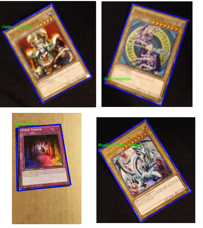
98% accuracy on the adversarial images after fine-tuning.

Let’s now go back and re-evaluate the CNN on both the original testing set and our adversarial images:

[INFO] normal testing images *after* fine-tuning:
[INFO] loss: 0.0594, acc: 0.9844

[INFO] adversarial images *after* fine-tuning:
[INFO] loss: 0.0366, acc: 0.9906

real	5m12.753s
user	12m42.125s
sys	10m0.498s

Initially, our CNN obtained 98.92% accuracy on our testing set. Accuracy has dropped on the testing set by \approx0.5%, but the good news is that we’re now hitting 99% accuracy when classifying our adversarial images, thereby implying that:

  1. Our model can make correct predictions on the original, non-perturbed images from the MNIST dataset.
  2. We can also make accurate predictions on the generated adversarial images (meaning that we’ve successfully defended against them).

How else can we defend against adversarial attacks?

Fine-tuning a model on adversarial images is just one way to defend against adversarial attacks.

A better way is to mix and incorporate adversarial images with the original images during the training process.

The result is a more robust model capable of defending against adversarial attacks since the model generates its own adversarial images in each batch, thereby continually improving itself rather than relying on a single round of fine-tuning after training.

We’ll be covering this “mixed batch adversarial training method” in next week’s tutorial.

Credits and references

The FGSM and data generator implementation were inspired by Sebastian Theiler’s excellent article on adversarial attacks and defenses. A huge shoutout and thank you to Sebastian for sharing his knowledge.

What’s next?

Figure 4: Join PyImageSearch University and learn Computer Vision using OpenCV and Python. Enjoy guided lessons, quizzes, assessments, and certifications. You’ll learn everything from deep learning foundations applied to computer vision up to advanced, real-time augmented reality. Don’t worry; it will be fun and easy to follow because I’m your instructor. Won’t you join me today to further your computer vision and deep learning study?

Would you enjoy learning how to successfully and confidently apply OpenCV to your projects?

Are you worried that configuring your development environment for Computer Vision, Deep Learning, and OpenCV will be too challenging, resulting in confusing, hard to debug error messages?

Concerned that you’ll get lost sifting through endless tutorials and video guides as you struggle to master Computer Vision?

No problem, because I’ve got you covered. PyImageSearch University is your chance to learn from me at your own pace.

You’ll find everything you need to master the basics (like we did together in this tutorial) and move on to advanced concepts.

Don’t worry about your operating system or development environment. I’ve got you covered with pre-configured Jupyter Notebooks in Google Colab for every tutorial on PyImageSearch, including Jupyter Notebooks for our new weekly tutorials as well!

Best of all, these Jupyter Notebooks will run on your machine, regardless of whether you are using Windows, macOS, or Linux! Irrespective of the operating system used, you will still be able to follow along and run the code in every lesson (all inside the convenience of your web browser).

Additionally, you can massively accelerate your progress by watching our video lessons accompanying each post. Every lesson at PyImageSearch University includes a detailed, step-by-step video guide.

You may feel that learning Computer Vision, Deep Learning, and OpenCV is too hard. Don’t worry; I’ll guide you gradually through each lecture and topic, so we build a solid foundation, and you grasp all the content.

When you think about it, PyImageSearch University is almost an unfair advantage compared to self-guided learning. You’ll learn more efficiently and master Computer Vision faster.

Oh, and did I mention you’ll also receive Certificates of Completion as you progress through each course at PyImageSearch University?

I’m sure PyImageSearch University will help you master OpenCV drawing and all the other computer vision skills you will need. Why not join today?

Summary

In this tutorial, you learned how to defend against adversarial image attacks using Keras and TensorFlow.

Our adversarial image defense worked by:

  1. Training a CNN on our dataset
  2. Generating a set of adversarial images using the trained model
  3. Fine-tuning our model on the adversarial images

The result is a model that is both:

  1. Accurate on the original testing images
  2. Capable of correctly classifying the adversarial images as well

The fine-tuning approach to adversarial image defense is essentially the most basic adversarial defense. Next week you’ll learn a more advanced method that incorporates batches of adversarial images generated on the fly, allowing the model to learn from the adversarial examples that “fooled” it during each epoch.

If you enjoyed this guide, you certainly wouldn’t want to miss next week’s tutorial!

To download the source code to this post (and be notified when future tutorials are published here on PyImageSearch), simply enter your email address in the form below!

Download the Source Code and FREE 17-page Resource Guide

Enter your email address below to get a .zip of the code and a FREE 17-page Resource Guide on Computer Vision, OpenCV, and Deep Learning. Inside you'll find my hand-picked tutorials, books, courses, and libraries to help you master CV and DL!

The post Defending against adversarial image attacks with Keras and TensorFlow appeared first on PyImageSearch.

Mixing normal images and adversarial images when training CNNs

$
0
0

In this tutorial, you will learn how to generate image batches of (1) normal images and (2) adversarial images during the training process. Doing so improves your model’s ability to generalize and defend against adversarial attacks.

Last week we learned a simple method to defend against adversarial attacks. This method was a simple three-step process:

  1. Train the CNN on your original training set
  2. Generate adversarial examples from the testing set (or equivalent holdout set)
  3. Fine-tune the CNN on the adversarial examples

This method works fine but can be vastly improved simply by altering the training process.

Instead of fine-tuning the network on a set of adversarial examples, we can alter the batch generation process itself.

When we train neural networks, we do so in batches of data. Each batch is a subset of the training data and is typically sized in powers of two (8, 16, 32, 64, 128, etc.). For each batch, we perform a forward pass of the network, compute the loss, perform backpropagation, and then update the network’s weights. This is the standard training protocol of essentially any neural network.

We can modify this standard training procedure to incorporate adversarial examples by:

  1. Initializing our neural network
  2. Selecting a total of N training examples
  3. Use the model and a method like FGSM to generate a total of N adversarial examples as well
  4. Combine the two sets, forming a batch of size Nx2
  5. Train the model on both the adversarial examples and original training samples

The benefit of this approach is that the model can learn from itself.

After each batch update, the model has improved by two factors. First, the model has ideally learned more discriminating patterns in the training data. Secondly, the model has learned to defend against adversarial examples that the model itself generated.

Throughout an entire training procedure (tens to hundreds of epochs with tens of thousands to hundreds of thousands of batch updates), the model naturally learns to defend itself against adversarial attacks.

This method is more complex than the basic fine-tuning approach, but the benefits dramatically outweigh the negatives.

To learn how to mix normal images with adversarial images during training to improve model robustness, just keep reading.

Looking for the source code to this post?

Jump Right To The Downloads Section

Mixing normal images and adversarial images when training CNNs

In the first part of this tutorial, we’ll learn how to mix normal images and adversarial images during the training process.

From there, we’ll configure our development environment and then review our project directory structure.

We’ll have several Python scripts to implement today, including:

  1. Our CNN architecture
  2. An adversarial image generator
  3. A data generator that (1) samples training data points and (2) generates adversarial examples on the fly
  4. A training script that puts all the pieces together

We’ll wrap up this tutorial by training our model on the mixed adversarial image generation process and then discuss the results.

Let’s get started!

How can we mix normal images and adversarial images during training?

Mixing training images with adversarial images is best explained visually. We start with both a neural network architecture and a training set:

Figure 1: To defend against adversarial attacks, we start with a neural network architecture and training set.

The normal training process works by sampling batches of data from the training set and then training the model:

Figure 2: The normal process of training.

However, we want to incorporate adversarial training, so we need a separate process that uses the model to generate adversarial examples:

Figure 3: To defend against adversarial attacks, we need to update our training procedure to sample batches of both normal training images and adversarial images (that are generated by the model during training).

Now, during our training process, we sample the training set and generate adversarial examples, and then train the network:

Figure 4: The full training process of mixing normal images and adversarial images together.

The training process is slightly more complex since we are sampling from our training set and generating adversarial examples on the fly. Still, the benefit is that the model can:

  1. Learn patterns from the original training set
  2. Learn patterns from the adversarial examples

Since the model has now been trained on adversarial examples, it will be more robust and generalize better when presented with adversarial images.

Configuring your development environment

This tutorial on defending against adversarial image attacks uses Keras and TensorFlow. If you intend to follow this tutorial, I suggest you take the time to configure your deep learning development environment.

You can utilize either of these two guides to install TensorFlow and Keras on your system:

Either tutorial will help you configure your system with all the necessary software for this blog post in a convenient Python virtual environment.

Having problems configuring your development environment?

Figure 5: Having trouble configuring your dev environment? Want access to pre-configured Jupyter Notebooks running on Google Colab? Be sure to join PyImageSearch University — you’ll be up and running with this tutorial in a matter of minutes.

All that said, are you:

  • Short on time?
  • Learning on your employer’s administratively locked system?
  • Wanting to skip the hassle of fighting with the command line, package managers, and virtual environments?
  • Ready to run the code right now on your Windows, macOS, or Linux systems?

Then join PyImageSearch University today!

Gain access to Jupyter Notebooks for this tutorial and other PyImageSearch guides that are pre-configured to run on Google Colab’s ecosystem right in your web browser! No installation required.

And best of all, these Jupyter Notebooks will run on Windows, macOS, and Linux!

Project structure

Let’s start this tutorial by reviewing our project directory structure.

Use the “Downloads” section of this guide to retrieve the source code. You’ll then be presented with the following directory:

$ tree . --dirsfirst
.
├── pyimagesearch
│   ├── __init__.py
│   ├── datagen.py
│   ├── fgsm.py
│   └── simplecnn.py
└── train_mixed_adversarial_defense.py

1 directory, 5 files

Our directory structure is essentially identical to last week’s tutorial on Defending against adversarial image attacks with Keras and TensorFlow. The primary difference is that:

  1. We’re adding a new function to our datagen.py file to handle mixing both training images and on-the-fly generated adversarial images at the same time.
  2. Our driver training script, train_mixed_adversarial_defense.py, has a few additional bells and whistles to handle mixed training.

If you haven’t yet, I strongly encourage you to read the previous two tutorials in this series:

  1. Adversarial attacks with FGSM (Fast Gradient Sign Method)
  2. Defending against adversarial image attacks with Keras and TensorFlow

They are considered required reading before you continue!

Our basic CNN

Our CNN architecture can be found inside the simplecnn.py file in our project structure. I’ve already reviewed this model definition in detail during our Fast Gradient Sign Method tutorial, so I’m going to defer a complete explanation of the code to that guide.

That said, I’ve included the full implementation of SimpleCNN for you to review below:

# import the necessary packages
from tensorflow.keras.models import Sequential
from tensorflow.keras.layers import BatchNormalization
from tensorflow.keras.layers import Conv2D
from tensorflow.keras.layers import Activation
from tensorflow.keras.layers import Flatten
from tensorflow.keras.layers import Dropout
from tensorflow.keras.layers import Dense

Lines 2-8 import our required Python packages.

We can then create the SimpleCNN architecture:

class SimpleCNN:
	@staticmethod
	def build(width, height, depth, classes):
		# initialize the model along with the input shape
		model = Sequential()
		inputShape = (height, width, depth)
		chanDim = -1

		# first CONV => RELU => BN layer set
		model.add(Conv2D(32, (3, 3), strides=(2, 2), padding="same",
			input_shape=inputShape))
		model.add(Activation("relu"))
		model.add(BatchNormalization(axis=chanDim))

		# second CONV => RELU => BN layer set
		model.add(Conv2D(64, (3, 3), strides=(2, 2), padding="same"))
		model.add(Activation("relu"))
		model.add(BatchNormalization(axis=chanDim))

		# first (and only) set of FC => RELU layers
		model.add(Flatten())
		model.add(Dense(128))
		model.add(Activation("relu"))
		model.add(BatchNormalization())
		model.add(Dropout(0.5))

		# softmax classifier
		model.add(Dense(classes))
		model.add(Activation("softmax"))

		# return the constructed network architecture
		return model

The salient points of this architecture include:

  1. A first set of CONV => RELU => BN layers. The CONV layer learns a total of 32 3×3 filters with 2×2 strided convolution to reduce volume size.
  2. A second set of CONV => RELU => BN layers. Same as above, but this time the CONV layer learns 64 filters.
  3. A set of dense/fully-connected layers. The output of which is our softmax classifier used for returning probabilities for each class label.

Using FGSM to generate adversarial images

We use the Fast Gradient Sign Method (FGSM) to generate image adversaries. We’ve covered this implementation in detail earlier in this series, so you can refer there for a complete review of the code.

That said, if you open the fgsm.py file in your project directory structure, you will find the following code:

# import the necessary packages
from tensorflow.keras.losses import MSE
import tensorflow as tf

def generate_image_adversary(model, image, label, eps=2 / 255.0):
	# cast the image
	image = tf.cast(image, tf.float32)

	# record our gradients
	with tf.GradientTape() as tape:
		# explicitly indicate that our image should be tacked for
		# gradient updates
		tape.watch(image)

		# use our model to make predictions on the input image and
		# then compute the loss
		pred = model(image)
		loss = MSE(label, pred)

	# calculate the gradients of loss with respect to the image, then
	# compute the sign of the gradient
	gradient = tape.gradient(loss, image)
	signedGrad = tf.sign(gradient)

	# construct the image adversary
	adversary = (image + (signedGrad * eps)).numpy()

	# return the image adversary to the calling function
	return adversary

At a high-level, this code is:

  1. Accepting a model that we want to “fool” into making incorrect predictions
  2. Taking the model and using it to make predictions on the input image
  3. Computing the loss of the model based on the ground-truth class label
  4. Computing the gradients of the loss with respect to the image
  5. Taking the sign of the gradient (either -1, 0, 1) and then using the signed gradient to create the image adversary

The end result will be an output image that looks visually identical to the original but that the CNN will classify incorrectly.

Again, you can refer to our FGSM guide for a detailed review of the code.

Updating our data generator to mix normal images with adversarial images on the fly

In this section, we are going to implement two functions:

  1. generate_adversarial_batch: Generates a total of N adversarial images using our FGSM implementation.
  2. generate_mixed_adverserial_batch: Generates a batch of N images, half of which are normal images and the other half are adversarial.

We implemented the first method last week in our tutorial on Defending against adversarial image attacks with Keras and TensorFlow. The second function is brand new and exclusive to this tutorial.

Let’s get started with our data batch generators. Open the datagen.py file in our project structure and insert the following code:

# import the necessary packages
from .fgsm import generate_image_adversary
from sklearn.utils import shuffle
import numpy as np

Lines 2-4 handle our required imports.

We’re importing the generate_image_adversary from our fgsm module such that we can generate image adversaries.

The shuffle function is imported to jointly shuffle images and labels together.

Below is the definition of our generate_adversarial_batch function, which we implemented last week:

def generate_adversarial_batch(model, total, images, labels, dims,
	eps=0.01):
	# unpack the image dimensions into convenience variables
	(h, w, c) = dims

	# we're constructing a data generator here so we need to loop
	# indefinitely
	while True:
		# initialize our perturbed images and labels
		perturbImages = []
		perturbLabels = []

		# randomly sample indexes (without replacement) from the
		# input data
		idxs = np.random.choice(range(0, len(images)), size=total,
			replace=False)

		# loop over the indexes
		for i in idxs:
			# grab the current image and label
			image = images[i]
			label = labels[i]

			# generate an adversarial image
			adversary = generate_image_adversary(model,
				image.reshape(1, h, w, c), label, eps=eps)

			# update our perturbed images and labels lists
			perturbImages.append(adversary.reshape(h, w, c))
			perturbLabels.append(label)

		# yield the perturbed images and labels
		yield (np.array(perturbImages), np.array(perturbLabels))

Since we discussed this function in detail in our previous post, I’m going to defer a complete discussion of the function to there, but at high-level, you can see that this function:

  1. Randomly samples N images (total) from our input images set (typically either our training or testing set)
  2. We then use the FGSM to generate adversarial examples from our randomly sampled images
  3. The function rounds out by returning the adversarial images and labels to the calling function

The big takeaway here is that the generate_adversarial_batch method returns exclusively adversarial images.

However, the goal of this post is mixed training containing both normal images and adversarial images. Therefore, we need to implement a second helper function:

def generate_mixed_adverserial_batch(model, total, images, labels,
	dims, eps=0.01, split=0.5):
	# unpack the image dimensions into convenience variables
	(h, w, c) = dims

	# compute the total number of training images to keep along with
	# the number of adversarial images to generate
	totalNormal = int(total * split)
	totalAdv = int(total * (1 - split))

As the name suggests, generate_mixed_adverserial_batch creates a mix of both normal images and adversarial images.

This method has several arguments, including:

  1. model: The CNN we’re training and using to generate adversarial images
  2. total: The total number of images we want in each batch
  3. images: The input set of images (typically either our training or testing split)
  4. labels: The corresponding class labels belonging to the images
  5. dims: The spatial dimensions of the input images
  6. eps: A small epsilon value used for generating the adversarial images
  7. split: Percentage of normal images vs. adversarial images; here, we are doing a 50/50 split

From there, we unpack the dims tuple into our height, width, and number of channels (Line 43).

We also derive the total number of training images and number of adversarial images based on our split (Lines 47 and 48).

Let’s now dive into the data generator itself:

	# we're constructing a data generator so we need to loop
	# indefinitely
	while True:
		# randomly sample indexes (without replacement) from the
		# input data and then use those indexes to sample our normal
		# images and labels
		idxs = np.random.choice(range(0, len(images)),
			size=totalNormal, replace=False)
		mixedImages = images[idxs]
		mixedLabels = labels[idxs]

		# again, randomly sample indexes from the input data, this
		# time to construct our adversarial images
		idxs = np.random.choice(range(0, len(images)), size=totalAdv,
			replace=False)

Line 52 starts an infinite loop that will continue until the training process is complete.

We then randomly sample a total of totalNormal images from our input set (Lines 56-59).

Next, Lines 63 and 64 perform a second round of random sampling, this time for adversarial image generation.

We can now loop over each of these idxs:

		# loop over the indexes
		for i in idxs:
			# grab the current image and label, then use that data to
			# generate the adversarial example
			image = images[i]
			label = labels[i]
			adversary = generate_image_adversary(model,
				image.reshape(1, h, w, c), label, eps=eps)

			# update the mixed images and labels lists
			mixedImages = np.vstack([mixedImages, adversary])
			mixedLabels = np.vstack([mixedLabels, label])

		# shuffle the images and labels together
		(mixedImages, mixedLabels) = shuffle(mixedImages, mixedLabels)

		# yield the mixed images and labels to the calling function
		yield (mixedImages, mixedLabels)

For each image index, i, we:

  1. Grab the current image and label (Lines 70 and 71)
  2. Generate an adversarial image via FGSM (Lines 72 and 73)
  3. Update our mixedImages and mixedLabels list with our adversarial image and label (Lines 76 and 77)

Line 80 jointly shuffles our mixedImages and mixedLabels. We perform this shuffling operation because the normal images and adversarial images were added together sequentially, meaning that the normal images appear at the front of the list while the adversarial images are at the back of the list. Shuffling ensures our data samples are randomly distributed throughout the batch.

The shuffled batch of data is then yielded to the calling function.

Creating our mixed image and adversarial image training script

With all of our helper functions implemented, we can create our training script.

Open the train_mixed_adverserial_defense.py file in your project structure, and let’s get to work:

# import the necessary packages
from pyimagesearch.simplecnn import SimpleCNN
from pyimagesearch.datagen import generate_mixed_adverserial_batch
from pyimagesearch.datagen import generate_adversarial_batch
from tensorflow.keras.optimizers import Adam
from tensorflow.keras.utils import to_categorical
from tensorflow.keras.datasets import mnist
import numpy as np

Lines 2-8 import our required Python packages. Take note of our custom implementations, including:

  1. SimpleCNN: The CNN architecture we’ll be training.
  2. generate_mixed_adverserial_batch: Generates batches of both normal images and adversarial images together
  3. generate_adversarial_batch: Generates batches of exclusively adversarial images

We’ll be training SimpleCNN on the MNIST dataset, so let’s load it and preprocess it now:

# load MNIST dataset and scale the pixel values to the range [0, 1]
print("[INFO] loading MNIST dataset...")
(trainX, trainY), (testX, testY) = mnist.load_data()
trainX = trainX / 255.0
testX = testX / 255.0

# add a channel dimension to the images
trainX = np.expand_dims(trainX, axis=-1)
testX = np.expand_dims(testX, axis=-1)

# one-hot encode our labels
trainY = to_categorical(trainY, 10)
testY = to_categorical(testY, 10)

Line 12 loads the MNIST digits dataset from disk. We then proceed to preprocess it by:

  1. Scaling the pixel intensities from the range [0, 255] to [0, 1]
  2. Adding a batch dimension to the data
  3. One-hot encoding the labels

We can now compile our model:

# initialize our optimizer and model
print("[INFO] compiling model...")
opt = Adam(lr=1e-3)
model = SimpleCNN.build(width=28, height=28, depth=1, classes=10)
model.compile(loss="categorical_crossentropy", optimizer=opt,
	metrics=["accuracy"])

# train the simple CNN on MNIST
print("[INFO] training network...")
model.fit(trainX, trainY,
	validation_data=(testX, testY),
	batch_size=64,
	epochs=20,
	verbose=1)

Lines 26-29 compile our model. We then train it on Lines 33-37 on our trainX and trainY data.

After training, the next step is to evaluate the model:

# make predictions on the testing set for the model trained on
# non-adversarial images
(loss, acc) = model.evaluate(x=testX, y=testY, verbose=0)
print("[INFO] normal testing images:")
print("[INFO] loss: {:.4f}, acc: {:.4f}\n".format(loss, acc))

# generate a set of adversarial from our test set (so we can evaluate
# our model performance *before* and *after* mixed adversarial
# training)
print("[INFO] generating adversarial examples with FGSM...\n")
(advX, advY) = next(generate_adversarial_batch(model, len(testX),
	testX, testY, (28, 28, 1), eps=0.1))

# re-evaluate the model on the adversarial images
(loss, acc) = model.evaluate(x=advX, y=advY, verbose=0)
print("[INFO] adversarial testing images:")
print("[INFO] loss: {:.4f}, acc: {:.4f}\n".format(loss, acc))

Lines 41-43 evaluate the model on our testing data.

We then generate a set of exclusively adversarial images on Lines 49 and 50.

Our model is then re-evaluated, this time on the adversarial images (Lines 53-55).

As we’ll see in the next section, our model will perform well on the original testing data, but accuracy will plummet on the adversarial images.

To help defend against adversarial attacks, we can fine-tune the model on data batches consisting of both normal images and adversarial examples.

The following code block accomplishes this task:

# lower the learning rate and re-compile the model (such that we can
# fine-tune it on the mixed batches of normal images and dynamically
# generated adversarial images)
print("[INFO] re-compiling model...")
opt = Adam(lr=1e-4)
model.compile(loss="categorical_crossentropy", optimizer=opt,
	metrics=["accuracy"])

# initialize our data generator to create data batches containing
# a mix of both *normal* images and *adversarial* images
print("[INFO] creating mixed data generator...")
dataGen = generate_mixed_adverserial_batch(model, 64,
	trainX, trainY, (28, 28, 1), eps=0.1, split=0.5)

# fine-tune our CNN on the adversarial images
print("[INFO] fine-tuning network on dynamic mixed data...")
model.fit(
	dataGen,
	steps_per_epoch=len(trainX) // 64,
	epochs=10,
	verbose=1)

Lines 61-63 lower our learning rate and then recompile our model.

From there, we create our data generator (Lines 68 and 69). Here we are telling our data generator to use our model to generate batches of data (with 64 total data points in each batch), sampling from our training data, with an equal 50/50 split for normal images and adversarial images.

Passing in our dataGen to model.fit allows our CNN to be trained on these mixed batches.

Let’s perform one final round of evaluation:

# now that our model is fine-tuned we should evaluate it on the test
# set (i.e., non-adversarial) again to see if performance has degraded
(loss, acc) = model.evaluate(x=testX, y=testY, verbose=0)
print("")
print("[INFO] normal testing images *after* fine-tuning:")
print("[INFO] loss: {:.4f}, acc: {:.4f}\n".format(loss, acc))

# do a final evaluation of the model on the adversarial images
(loss, acc) = model.evaluate(x=advX, y=advY, verbose=0)
print("[INFO] adversarial images *after* fine-tuning:")
print("[INFO] loss: {:.4f}, acc: {:.4f}".format(loss, acc))

Lines 81-84 evaluate our CNN on our original testing set after fine-tuning on mixed batches.

We then evaluate the CNN on our original adversarial images once again (Lines 87-89).

Ideally, what we’ll see is balanced accuracy between our normal images and adversarial images, thus making our model more robust and capable of defending against an adversarial attack.

Training our CNN on normal images and adversarial images

We are now ready to train our CNN on both normal training images and adversarial images generated on the fly.

Start by accessing the “Downloads” section of this tutorial to retrieve the source code.

From there, open a terminal and execute the following command:

$ time python train_mixed_adversarial_defense.py
[INFO] loading MNIST dataset...
[INFO] compiling model...
[INFO] training network...
Epoch 1/20
938/938 [==============================] - 6s 6ms/step - loss: 0.2043 - accuracy: 0.9377 - val_loss: 0.0615 - val_accuracy: 0.9805
Epoch 2/20
938/938 [==============================] - 6s 6ms/step - loss: 0.0782 - accuracy: 0.9764 - val_loss: 0.0470 - val_accuracy: 0.9846
Epoch 3/20
938/938 [==============================] - 6s 6ms/step - loss: 0.0597 - accuracy: 0.9810 - val_loss: 0.0493 - val_accuracy: 0.9828
...
Epoch 18/20
938/938 [==============================] - 6s 6ms/step - loss: 0.0102 - accuracy: 0.9965 - val_loss: 0.0478 - val_accuracy: 0.9889
Epoch 19/20
938/938 [==============================] - 6s 6ms/step - loss: 0.0116 - accuracy: 0.9961 - val_loss: 0.0359 - val_accuracy: 0.9915
Epoch 20/20
938/938 [==============================] - 6s 6ms/step - loss: 0.0105 - accuracy: 0.9967 - val_loss: 0.0477 - val_accuracy: 0.9891
[INFO] normal testing images:
[INFO] loss: 0.0477, acc: 0.9891

Above, you can see the output of training our CNN on the normal MNIST training set. Here, we obtain 99.67% accuracy on the training set and 98.91% accuracy on the testing set.

Now, let’s see what happens when we generate a set of adversarial images with the Fast Gradient Sign Method:

[INFO] generating adversarial examples with FGSM...

[INFO] adversarial testing images:
[INFO] loss: 14.0658, acc: 0.0188

Our accuracy plummets from 98.91% accuracy down to 1.88% accuracy. Clearly, our model is not handling adversarial examples well.

What we’ll do now is lower the learning rate, re-compile the model, and then fine-tune using a data generator that includes both the original training images and adversarial images generated on the fly:

[INFO] re-compiling model...
[INFO] creating mixed data generator...
[INFO] fine-tuning network on dynamic mixed data...
Epoch 1/10
937/937 [==============================] - 162s 173ms/step - loss: 1.5721 - accuracy: 0.7653
Epoch 2/10
937/937 [==============================] - 146s 156ms/step - loss: 0.4189 - accuracy: 0.8875
Epoch 3/10
937/937 [==============================] - 146s 156ms/step - loss: 0.2861 - accuracy: 0.9154
...
Epoch 8/10
937/937 [==============================] - 146s 155ms/step - loss: 0.1423 - accuracy: 0.9541
Epoch 9/10
937/937 [==============================] - 145s 155ms/step - loss: 0.1307 - accuracy: 0.9580
Epoch 10/10
937/937 [==============================] - 146s 155ms/step - loss: 0.1234 - accuracy: 0.9604

Using this approach, we obtain 96.04% accuracy.

And when we apply it to our final testing images, we arrive at the following:

[INFO] normal testing images *after* fine-tuning:
[INFO] loss: 0.0315, acc: 0.9906

[INFO] adversarial images *after* fine-tuning:
[INFO] loss: 0.1190, acc: 0.9641

real    27m17.243s
user    43m1.057s
sys     14m43.389s

After fine-tuning our model using the dynamic data generation process, we obtain 99.06% accuracy on the original testing images (up from 98.44% from last week’s method).

Our adversarial image accuracy weighs in at 96.41%, which is down from 99% last week, but that makes sense in this context — keep in mind that we are not fine-tuning the model on just the adversarial examples like we did last week. Instead, we allow the model to “iteratively fool itself” and learn from the adversarial examples that it generates.

Further accuracy could potentially be obtained by fine-tuning again on only the adversarial examples (without any original training samples). Still, I’ll leave that as an exercise for you, the reader, to explore.

Credits and references

The FGSM and data generator implementation were inspired by Sebastian Theiler’s excellent article on adversarial attacks and defenses. A huge shoutout and thank you to Sebastian for sharing his knowledge.

What’s next?

Figure 6: Join PyImageSearch University and learn Computer Vision using OpenCV and Python. Enjoy guided lessons, quizzes, assessments, and certifications. You’ll learn everything from deep learning foundations applied to computer vision up to advanced, real-time augmented reality. Don’t worry; it will be fun and easy to follow because I’m your instructor. Won’t you join me today to further your computer vision and deep learning study?

Would you enjoy learning how to successfully and confidently apply OpenCV to your projects?

Are you worried that configuring your development environment for Computer Vision, Deep Learning, and OpenCV will be too challenging, resulting in confusing, hard to debug error messages?

Concerned that you’ll get lost sifting through endless tutorials and video guides as you struggle to master Computer Vision?

No problem, because I’ve got you covered. PyImageSearch University is your chance to learn from me at your own pace.

You’ll find everything you need to master the basics (like we did together in this tutorial) and move on to advanced concepts.

Don’t worry about your operating system or development environment. I’ve got you covered with pre-configured Jupyter Notebooks in Google Colab for every tutorial on PyImageSearch, including Jupyter Notebooks for our new weekly tutorials as well!

Best of all, these Jupyter Notebooks will run on your machine, regardless of whether you are using Windows, macOS, or Linux! Irrespective of the operating system used, you will still be able to follow along and run the code in every lesson (all inside the convenience of your web browser).

Additionally, you can massively accelerate your progress by watching our video lessons accompanying each post. Every lesson at PyImageSearch University includes a detailed, step-by-step video guide.

You may feel that learning Computer Vision, Deep Learning, and OpenCV is too hard. Don’t worry; I’ll guide you gradually through each lecture and topic, so we build a solid foundation and you grasp all the content.

When you think about it, PyImageSearch University is almost an unfair advantage compared to self-guided learning. You’ll learn more efficiently and master Computer Vision faster.

Oh, and did I mention you’ll also receive Certificates of Completion as you progress through each course at PyImageSearch University?

I’m sure PyImageSearch University will help you master OpenCV drawing and all the other computer vision skills you will need. Why not join today?

Summary

In this tutorial, you learned how to modify a CNN’s training procedure to generate image batches that include:

  1. Normal training images
  2. Adversarial examples generated by the CNN

This method is different from the one we learned last week, where we simply fine-tuned a CNN on a sample of adversarial images.

The benefit of today’s approach is that the CNN can better defend against adversarial examples by:

  1. Learning patterns from the original training examples
  2. Learning patterns from the adversarial images generated on the fly

Since the model can generate its own adversarial examples during every batch of training, it can continually learn from itself.

Overall, I think you’ll find this approach more beneficial when training your own models to defend against adversarial attacks.

To download the source code to this post (and be notified when future tutorials are published here on PyImageSearch), simply enter your email address in the form below!

Download the Source Code and FREE 17-page Resource Guide

Enter your email address below to get a .zip of the code and a FREE 17-page Resource Guide on Computer Vision, OpenCV, and Deep Learning. Inside you'll find my hand-picked tutorials, books, courses, and libraries to help you master CV and DL!

The post Mixing normal images and adversarial images when training CNNs appeared first on PyImageSearch.

An interview with Jagadish Mahendran, 1st place winner of the OpenCV Spatial AI Competition

$
0
0

In this post, I interview Jagadish Mahendran, senior Computer Vision/Artificial Intelligence (AI) engineer who recently won 1st place in the OpenCV Spatial AI Competition using the new OpenCV AI Kit (OAK).

Jagadish’s winning project was a computer vision system for the visually impaired, allowing users to successfully and safely navigate the world. His project included:

  • Automatic detection of crosswalks
  • Crosswalk and stop sign detection
  • Overhanging obstacle detection
  • …and more!

Best of all, this entire project was built around the new OpenCV Artificial Intelligence Kit (OAK), an embedded device designed specifically for computer vision.

Join me in learning about Jagadish’s project and how he uses computer vision to help visually impaired people.

An interview with Jagadish Mahendran, 1st place winner of the OpenCV Spatial AI Competition

Adrian: Welcome, Jagadish! Thank you so much for being here. It’s a pleasure to have you on the PyImageSearch blog.

Jagadish: Pleasure to be interviewed by you, Adrian. Thanks for having me.


Adrian: Before we get started, can you tell us a bit about yourself? Where do you work, and what is your role there?

Jagadish: I am a senior Computer Vision / Artificial Intelligence (AI) engineer. I have worked for multiple startups, where I have built AI and perception solutions for inventory management robots and cooking robots.


Figure 1: Jagadish participated in the 2020 OpenCV Spatial AI Competition and won first place (image source).

Adrian: How did you first become interested in computer vision and robotics?

Jagadish: I have been interested in AI since my undergraduate studies, where I had an opportunity to build a micromouse robot with my friends. I got attracted to computer vision and machine learning during my Master’s. Since then, it has been great fun working with these amazing technologies.


Adrian: You recently won 1st place in the OpenCV Spatial AI Competition, congratulations! Can you give us more details on the competition? How many teams participated, and what was the end goal of the contest?

Jagadish: Thank you. The OpenCV Spatial AI 2020 Competition sponsored by Intel involved 2 phases. Around 235 teams with various backgrounds, including university labs and companies, participated in Phase 1, which involved proposing an idea that solves a real-world problem using an OpenCV AI Kit with Depth (OAK-D) sensor. Thirty-one teams were selected for Phase 2, where we had to implement our ideas for 3 months. The end goal is to develop a fully functioning AI system using an OAK-D sensor.


Adrian: Your winning solution was a vision system for the visually impaired. Can you tell us more about your project?

Jagadish: There are various visual assistance systems available in the literature and even in the market. Most of them don’t use deep learning methods due to hardware limitations, cost, and other challenges. But recently, there has been significant improvement in edge AI and sensor space which I thought could provide deep learning support to the visual assistance system with limited hardware.

I developed a wearable visual assistance system that uses an OAK-D sensor for perception, external neural compute sticks (NCS2), and my 5-year-old laptop for computing. The system can perform various computer vision tasks that can help visually impaired people with scene understanding.

These tasks include: detecting obstacles; elevation changes; and understanding road, sidewalk, and traffic conditions.

The system can detect traffic signs along with many other classes like people, cars, bicycles, and so on. The system can also detect obstacles using point clouds and update the individual regarding their presence using a voice interface. The individual can also interact with the system using a speech recognition system.

Here are a few sample outputs:

Figure 2: Jagadish’s project can detect stop signs, crosswalks, low-hanging objects, vehicles, bicycles, pedestrians, and more.

Figure 3: The OpenCV AI Kit with depth computation (image source).

Adrian: Tell us about the hardware used to develop your project submission. Does the individual need to wear a lot of bulky hardware and devices?

Jagadish: I interviewed a few visually impaired people and learned that getting too much attention while walking on the streets is one of the major issues faced by the visually impaired. So the physical system not being noticeable as an assistive device was a major goal. The developed system is simple — the physical setup includes my 5-year-old laptop, 2 neural compute sticks, camera hidden inside a cotton vest, GPS, and if needed, an additional camera can be placed inside a fanny pack/waist bag. Most of these devices are nicely packaged inside a backpack. Overall it looks like a college student walking around wearing a vest. I have walked around my downtown area, drawing absolutely no special attention.


Adrian: Why did you choose the OpenCV AI Kit (OAK), and more specifically, the OAK-D module that can compute depth information?

Jagadish: The organizers provided OAK-D as part of the competition, and it has many benefits. It is small. Along with RGB images, it can also provide depth images. These depth images have been very useful to detect obstacles even without knowing what obstacle it is. Also, it has an on-chip AI processor, which means computer vision tasks are already performed before the frames reach the host. This makes the system superfast.


Adrian: Do you have any demos of your vision system for visual impairment in action?

Jagadish: Demos can be found here:


Adrian: I noticed that your system has GPS as well as vision components. Why was it necessary to include GPS?

Jagadish: I wanted the system to be comprehensive, reliable, and also expandable. So I tried to include as many supplemental features as possible. GPS has been a great addition in that regard. It is a mature technology that is cheap and easy to set up. It can help with localization without the need for advanced robotics navigation and perception algorithms. I also wanted the GPS feature to be used differently from the usual map services. So I added a feature to save preferred locations, like a friend’s place, the gym, or a grocery store using custom names. The user can request the system for distances to these saved locations utilizing a voice recognition system. Also, the GPS location can be shared with preferred contacts via SMS.


Adrian: What was the biggest challenge developing the vision system for the visually impaired?

Jagadish: From a developer’s perspective, it is a complex system that involves both hardware and AI components. There was a lot of trial and error involved in choosing the harness for the sensors. Dataset collection and testing process required hours of walking in different areas of the town and at various times of the day. For deep learning, the biggest challenge was choosing models that are lighter with high accuracy and getting all these models working together in real-time on limited hardware.


Adrian: If you had to pick the most important technique you applied when developing the project, what would it be?

Jagadish: Model quantization techniques can provide a huge boost to inference speed with acceptable compromise in accuracy. OpenVINO optimizations were able to boost inference speed sometimes by up to \approx13x. Lighter models can learn faster/better from smaller images. For example, the MobileNetV2 object detection model trained on 300×300 images performed better than 450×450 images.


Adrian: What are the next steps for the project? Will you continue to develop it?

Jagadish: The next immediate step I am currently working on is getting the project tested by my visually impaired friend. I will ship the system to her soon. Also, there are numerous new features in the pipeline to be added. I am also working on making the project open source and mainstream. The idea is anyone should be able to use the complete AI stack for free, provided they can buy the sensors and computing unit on their own. I am also trying to build a developer’s community. So far, I have received some positive responses on this. Hopefully, the project becomes self-maintained in the future. We are also planning to obtain some funds for project expansion. I hope the project will make life easier for the visually impaired and increase their engagement in daily activities.


Adrian: What are your computer vision and deep learning tools, libraries, and packages of choice?

Jagadish: OpenCV for image manipulations and operations. Tensorflow, Keras, and PyTorch were used for deep learning. For edge AI – OpenVINO, TensorflowLite. DepthAI for OAK-D. Open3D for point cloud processing. Vosk for speech recognition, Festival for text-to-speech. Apart from them, standard python packages such as numpy, pandas, sklearn, etc., were used.


Adrian: What advice would you give to someone who wants to follow in your footsteps but doesn’t know how to get started?

Jagadish: AI can be deceiving. It is easy to get started and quickly gain a sense of mastery. However, this is not necessarily true. We are usually only touching the tip of the iceberg. There is a lot more going on in the background, even with a simple sigmoid activation function. It helps to learn systematically from the basics, solving practical and diverse problems, rather than just reading. Also, the AI community is very active and continuously evolving. It helps to read papers.


Adrian: You’ve been a PyImageSearch reader and customer since 2016! Thank you for supporting PyImageSearch and me. What PyImageSearch books and courses do you own? And how did they help prepare you for this competition?

Jagadish: I have been a PyImageSearch reader since my student life. I follow your blog posts regularly. I own the Practical Python and OpenCV book, complete ImageNet Bundle of Deep Learning for Computer Vision with Python, Complete Bundle of Raspberry Pi for Computer Vision. I will be grabbing the OCR bundle at some point. I have also completed the PyImageSearch Gurus course. I am currently trying out PyImageSearch University.

The PyImageSearch content, in general, has helped me with my professional career. In the competition, techniques from blogs and course materials were used to train lighter models to obtain faster and more accurate models. For example, the TrafficSignNet model from the traffic sign classification blog was used to classify images with traffic signs and other classes. MiniVGGNet from the deep learning bundle was trained to detect elevation changes from depth images.

Congratulations and thanks for making such quality content, Adrian.


Adrian: Would you recommend these books and courses to other budding developers, students, and researchers trying to learn computer vision, deep learning, and OpenCV?

Jagadish: Yes, absolutely.


Adrian: If a PyImageSearch reader wants to chat about your project, what is the best place to connect with you?

Jagadish: Happy to connect on LinkedIn — https://www.linkedin.com/in/jagadish-mahendran/

Summary

In this blog post, we interviewed Jagadish Mahendran, who won 1st place in the OpenCV Spatial AI Competition.

Jagadish is doing amazing work that can help visually impaired people — and doing so using hardware that makes computer vision and deep learning easy to apply.

I’m excited to follow Jagadish’s work, and I wish him the best of luck continuing to develop it.

To be notified when future tutorials and interviews are published here on PyImageSearch, simply enter your email address in the form below!

Download the Source Code and FREE 17-page Resource Guide

Enter your email address below to get a .zip of the code and a FREE 17-page Resource Guide on Computer Vision, OpenCV, and Deep Learning. Inside you'll find my hand-picked tutorials, books, courses, and libraries to help you master CV and DL!

The post An interview with Jagadish Mahendran, 1st place winner of the OpenCV Spatial AI Competition appeared first on PyImageSearch.

An interview with Gary Song, deep learning practitioner at Unity Technologies

$
0
0

In this blog post, I interview Gary Song, a deep learning practitioner at Unity Technologies.

We’re now at the one-year anniversary of COVID-19. It’s been a particularly rough year for all of us. For Gary, it was really bad.

But as his story shows, there are always ways to turn lemons into lemonade … if you’re willing to put in the hard work.

In 2020, Gary was managing a family emergency, and right as he returned home, COVID-19 struck. The economy went into a tailspin. The pandemic was especially hard on his employer, resulting in tremendous pay cuts.

Anxious about his future, both financially and professionally, Gary worked hard studying computer vision and deep learning. He created projects that demonstrated his knowledge of the field. And he put his resume out there, even though hiring conditions were tough.

In short, Gary invested in himself — and despite a worldwide pandemic going on, he landed a deep learning practitioner position at one of the world’s most famous video game companies.

I love sharing stories like Gary’s. I’m a firm believer that every person on this earth is the master of their own destiny … but in order to achieve your full potential, you need to put in the hard work.

A little luck doesn’t help either, but as one of my favorite sayings goes:

Fortune favors hard workers.

It’s amazing to see how far the world has fallen in one year — but it’s equally incredible to see how fast we’re recovering. It’s anyone’s guess when things will return to “normal” (or whatever the new version of normal is), but given that we’re now at the one-year anniversary of COVID-19, I couldn’t think of a better, more inspirational story to share.

Join me in learning how Gary Song landed a deep learning job at one of the world’s most famous video game companies, despite a worldwide pandemic going on.

An interview with Gary Song, deep learning practitioner at Unity Technologies

Adrian: Hi Gary! Thank you for taking the time to do this interview. I know you’re busy with your new job. It’s a pleasure to have you on the PyImageSearch blog.

Gary: Hey Adrian! The pleasure’s all mine.

Figure 1: Gary suffered substantial pay cuts at his old position during COVID-19. He used it as a catalyst to find and land a job in the deep learning field.

Adrian: COVID has made the past year really hard on people and businesses. How did COVID impact you and your job?

Gary: I definitely went through a rough stretch at the beginning of the year. I had just returned from a family emergency overseas, and COVID pretty much hit right after I came back. My then employer was affected pretty much immediately, and pay cuts came swiftly. I was thankful to be still employed, but with only uncertainty ahead, the stress and anxiety quickly became overbearing.

Figure 2: Gary Song now works at Unity Technologies as a deep learning practitioner.

Adrian: After the pay cuts, you ended up leaving your old job, and during a worldwide pandemic, you landed a new job as a deep learning practitioner at Unity Technologies, a video game software development company. That’s amazing. Congratulations! Can you walk us through that process? How did you have the courage to leave your job during COVID and then land this amazing position?

Gary: Thanks! Absolutely. So the first thing I remember was the hiring bar suddenly going up everywhere. Many places stopped hiring for junior and intermediate positions, and existing offers were being rescinded. Even in that climate, I knew that settling for a job just to be employed could easily be a death sentence for my career, so I had to be somewhat selective.

The way I tried to make my resume stand out was to highlight the fact that I had quickly built a prototype leveraging computer vision and deep learning to solve an existing business problem. That probably helped a lot in getting interviews.

I knew I was well prepared for those interviews because I had hands-on experience and knowledge of the nuances of working with deep learning models from working through the PyImageSearch courses and reading the blog. That, I think, was the differentiator.

I mean, anyone with a semester of multivariate calculus can answer some general questions about deep learning, ya know? But it takes the experience of preparing the data, training the models, debugging and improving bad results, etc., all of which your materials cover, to really know it well.

Now, I did always have to make it clear that my experience up to that point was solely with the computer vision applications of deep learning, but the knowledge was definitely transferrable, being applicable even in my current day-to-day work.


Adrian: What are your day-to-day responsibilities at Unity? What types of deep learning models are you working with?

Figure 3: Unity’s perception toolkit has been used to generate synthetic image data for object detection and image segmentation.

Gary: It’s essentially a cycle of meeting with stakeholders and structuring the project around the business requirements, then understanding the data and iterating on the model.

For example, I’m currently working on a churn prediction project. Although it’s fairly well known that gradient boosting algorithms tend to beat simple deep learning models on tabular data, I still get to use deep learning to understand the data and complement the results of the gradient boosting models.

As an example, latent space features from a very deep multi-task model can be used to look for objective-aware clusters to help us better understand our customers, which is important beyond the scope of this project.

Because my role is on the business side of things, I don’t often encounter unstructured data like images, so unless there’s a business case, I won’t get to do much computer vision in this particular role. However, I know that we have been very successful with our perception toolkit for generating synthetic data for object detection and image segmentation. It’s very cool, and I recommend everyone to check it out!


Adrian: What was your background in computer vision and deep learning before you joined Unity?

Gary: My knowledge of computer vision was just everything I learned in the PyImageSearch Gurus class, plus a few things I picked up on my own doing projects.

On the other hand, I knew deep learning fundamentals and major developments well, could implement models from papers from scratch, knew how to customize existing model architectures, and had a good sense of the effectiveness of models for given business use cases.

The deep learning fundamentals were from taking some online classes, reading books, watching lecture videos, and reading papers. Most of the implementation experience, however, came from following the Deep Learning for Computer Vision with Python ImageNet bundle.

Once I understood each model’s components, I started reading the papers cited in the books to understand the implementation details. Another thing I like about the PyImageSearch books is that they cite the original research papers, whereas a lot of online courses don’t do that.


Adrian: How did you first become interested in computer vision and deep learning?

Gary: I think the first time I encountered computer vision and deep learning together at the nuts and bolts level was in 2018 when my good friend and then colleague Jing Wang experimented with it.

Since deep learning has been trending as one of the most disruptive technologies over the last few years, I naturally wanted to learn it, but with new technologies, it’s never clear if it’s worth the time investment to learn if you’ve only heard about it. So, seeing someone at work use it made it clear that adding this to my toolkit was something I should prioritize.

I chose computer vision as my entry point to deep learning because computer vision seemed to be very intuitive, so it’s much easier to come up with hypotheses and applications for the technology.


Adrian: Do you have any recommendations for readers who want to follow in your footsteps?

Gary: I can definitely speak to this. Deep learning wasn’t offered in any courses back when I was in school, so I don’t have a very deep academic background in deep learning. As such, most of this advice is for aspiring practitioners in the industry, i.e., this is about eventually getting a role where deep learning is a staple part of your job. In no particular order:

  • Keep an eye on developments in the hardware space. Certain things may be done now due to computational constraints but may become less relevant once the hardware is powerful enough. Certain models may also just be out of reach for the average practitioner with access to only consumer-grade hardware. Due to the experiment-heavy nature of deep learning in practice, this can severely limit what you can afford to study, even if you use cloud resources. This was one reason I chose computer vision rather than NLP, as cutting-edge NLP models have grown incredibly big and hence, cost-prohibitive to experiment with.
  • Don’t hesitate to invest in computing power, whether it’s hardware or cloud. Computing power will let you experiment faster so that you learn faster.
  • Don’t hesitate to invest in courses that walk you through the end-to-end deep learning pipeline. Good courses that walk you through the end-to-end deep learning pipeline will save you time so that you can focus on the part you want to study. Also, it’s generally better to have a curriculum and all the information in one place rather than you having to dig through various sources on the web.
  • Build something and think about how to scale it. The modeling process is usually only part of the job. The point is that you want to demonstrate a capacity to handle all aspects of a project. This isn’t necessarily something specific to deep learning, but something employers will care about.
  • Read source code. There are lots to be learned from good implementations, including how to think about a problem and its solution.
  • Read at least one paper and implement the model from scratch. The devil is in the details. You’ll get a much deeper understanding of the principles behind model architectures in general.
  • In general, try to dedicate time to deep dives into your topic of interest. Out-of-the-box solutions will only take you so far and can be used as quick and dirty baselines, but it is only through these deep dives that you’ll understand how to improve your results.

Finally, here is some advice from Andrej Karpathy that I’ve taken to heart regarding becoming an expert:

Figure 4: Advice on how to become an expert (image source).

Adrian: You’ve been a PyImageSearch reader and customer since June 2019! Thank you for supporting PyImageSearch and me. What PyImageSearch books and courses do you own? And how did they help prepare for your new job at Unity?

Gary: I actually own all of them, except for the OCR one, which I’m going to get for a side project. The books and courses served as guided labs where I could get hands-on experience and become comfortable with all parts of the deep learning pipeline, which is important in the industry.

These materials were really my introduction to the “real” world of deep learning outside of a theory and derivations-heavy class. As such, they served as a survey of the landscape of deep learning by not only covering the models but also the datasets that are used to benchmark against.

Some of you might’ve heard of the notion that when learning a new subject, it’s important to build a “zoo,” as in, to be aware of, and to understand the interesting and illustrative cases. This is essentially what the PyImageSearch books and courses do for you.


Adrian: Would you recommend these books and courses to other budding developers, students, and researchers trying to learn computer vision, deep learning, and OpenCV?

Gary: 100%! I think these books and courses are tremendously valuable, especially for the demographic I’m in.

When I was in school, there weren’t any classes for deep learning, so I never got an opportunity to build a mental model of how everything fits together. With these books and courses, I was able to do that.

I recommend getting started with the Deep Learning for Computer Vision with Python ImageNet bundle. It can be used as guided deep learning labs or as a reference. The code is also very helpful because official documentation can be incomplete or, even worse, can have a scope that exceeds your needs, miring you with information overload.

Lastly, but perhaps most importantly, it is dense in practical knowledge not often mentioned elsewhere.


Adrian: If a PyImageSearch reader wants to connect with you, what is the best place to connect with you?

Gary: I’m always available on LinkedIn or through PyImageSearch direct messaging. I look forward to connecting with everyone!

Summary

In this blog post, we interviewed Gary Song, a deep learning practitioner at the famous video game development company, Unity Technologies.

Gary landed his deep learning position at Unity in the middle of the COVID-19 pandemic. He used the pay cuts at his previous job as motivation to study, improve himself, and land a position that he was not only proud of, but more stable as well.

I’m so incredibly proud of Gary. He’s put in the hard work, and he’s now enjoying the fruits of his labor.

Remember, fortune favors hard workers — are you working hard? Or hardly working?

To download the source code to this post (and be notified when future tutorials are published here on PyImageSearch), simply enter your email address in the form below!

Join the PyImageSearch Newsletter and Grab My FREE 17-page Resource Guide PDF

Enter your email address below to join the PyImageSearch Newsletter and download my FREE 17-page Resource Guide PDF on Computer Vision, OpenCV, and Deep Learning.

The post An interview with Gary Song, deep learning practitioner at Unity Technologies appeared first on PyImageSearch.


What is Deep Learning?

$
0
0

Deep learning methods are representation-learning methods with multiple levels of representation, obtained by composing simple but nonlinear modules that each transform the representation at one level (starting with the raw input) into a representation at a higher, slightly more abstract level. [. . . ] The key aspect of deep learning is that these layers are not designed by human engineers: they are learned from data using a general-purpose learning procedure.

Yann LeCun, Yoshua Bengio, and Geoffrey Hinton, Nature (2015), p. 436

Deep learning is a subfield of machine learning, which is, in turn, a subfield of artificial intelligence (AI). For a graphical depiction of this relationship, please refer to Figure 1.

Figure 1: A Venn diagram describing deep learning as a subfield of machine learning which, in turn, is a subfield of artificial intelligence (Image inspired by Figure 1.4 of Goodfellow et al., 2016).

The central goal of AI is to provide a set of algorithms and techniques that can be used to solve problems that humans perform intuitively and near automatically, but are otherwise very challenging for computers. A great example of such a class of AI problems is interpreting and understanding the contents of an image — this task is something that a human can do with little-to-no effort, but it has proven to be extremely difficult for machines to accomplish.

While AI embodies a large, diverse set of work related to automatic machine reasoning (inference, planning, heuristics, etc.), the machine learning subfield tends to be specifically interested in pattern recognition and learning from data.

Artificial Neural Networks (ANNs) are a class of machine learning algorithms that learn from data and specialize in pattern recognition, inspired by the structure and function of the brain. As we’ll find out, deep learning belongs to the family of ANN algorithms, and in most cases, the two terms can be used interchangeably. In fact, you may be surprised to learn that the deep learning field has been around for over 60 years, going by different names and incarnations based on research trends, available hardware and datasets, and popular options of prominent researchers at the time.

In the remainder of this chapter, we’ll review a brief history of deep learning, discuss what makes a neural network “deep,” and discover the concept of “hierarchical learning” and how it has made deep learning one of the major success stories in modern day machine learning and computer vision.

A Concise History of Neural Networks and Deep Learning

The history of neural networks and deep learning is a long, somewhat confusing one. It may surprise you to know that “deep learning” has existed since the 1940s undergoing various name changes, including cybernetics, connectionism, and the most familiar, Artificial Neural Networks (ANNs).

While inspired by the human brain and how its neurons interact with each other, ANNs are not meant to be realistic models of the brain. Instead, they are an inspiration, allowing us to draw parallels between a very basic model of the brain and how we can mimic some of this behavior through artificial neural networks.

The first neural network model came from McCulloch and Pitts in 1943. This network was a binary classifier, capable of recognizing two different categories based on some input. The problem was that the weights used to determine the class label for a given input needed to be manually tuned by a human — this type of model clearly does not scale well if a human operator is required to intervene.

Then, in the 1950s the seminal Perceptron algorithm was published by Rosenblatt (1958, 1962) — this model could automatically learn the weights required to classify an input (no human intervention required). An example of the Perceptron architecture can be seen in Figure 2. In fact, this automatic training procedure formed the basis of Stochastic Gradient Descent (SGD) which is still used to train very deep neural networks today.

Figure 2: An example of the simple Perceptron network architecture that accepts a number of inputs, computes a weighted sum, and applies a step function to obtain the final prediction.

During this time period, Perceptron-based techniques were all the rage in the neural network community. However, a 1969 publication by Minsky and Papert effectively stagnated neural network research for nearly a decade. Their work demonstrated that a Perceptron with a linear activation function (regardless of depth) was merely a linear classifier, unable to solve nonlinear problems. The canonical example of a nonlinear problem is the XOR dataset in Figure 3. Take a second now to convince yourself that it is impossible to try a single line that can separate the blue stars from the red circles.

Figure 3: The XOR (E(X)clusive Or) dataset is an example of a nonlinear separable problem that the Perceptron cannot solve. Take a second to convince yourself that it is impossible to draw a single line that separates the blue stars from the red circles.

Furthermore, the authors argued that (at the time) we did not have the computational resources required to construct large, deep neural networks (in hindsight, they were absolutely correct). This single paper alone almost killed neural network research.

Luckily, the backpropagation algorithm and the research by Werbos (1974), Rumelhart et al. (1986), and LeCun et al. (1998) were able to resuscitate neural networks from what could have been an early demise. Their research in the backpropagation algorithm enabled multi-layer feedforward neural networks to be trained (Figure 4).

Figure 4: A multi-layer, feedforward network architecture with an input layer (3 nodes), two hidden layers (2 nodes in the first layer and 3 nodes in the second layer), and an output layer (2 nodes).

Combined with nonlinear activation functions, researchers could now learn nonlinear functions and solve the XOR problem, opening the gates to an entirely new area of research in neural networks. Further research demonstrated that neural networks are universal approximators, capable of approximating any continuous function (but placing no guarantee on whether or not the network can actually learn the parameters required to represent a function).

The backpropagation algorithm is the cornerstone of modern day neural networks allowing us to efficiently train neural networks and “teach” them to learn from their mistakes. But even so, at this time, due to (1) slow computers (compared to modern day machines) and (2) lack of large, labeled training sets, researchers were unable to (reliably) train neural networks that had more than two hidden layers — it was simply computationally infeasible.

Today, the latest incarnation of neural networks as we know it is called deep learning. What sets deep learning apart from its previous incarnations is that we have faster, specialized hardware with more available training data. We can now train networks with many more hidden layers that are capable of hierarchical learning where simple concepts are learned in the lower layers and more abstract patterns in the higher layers of the network.

Perhaps the quintessential example of applied deep learning to feature learning is the Convolutional Neural Network (LeCun et al., 1998) applied to handwritten character recognition which automatically learns discriminating patterns (called “filters”) from images by sequentially stacking layers on top of each other. Filters in lower levels of the network represent edges and corners, while higher-level layers use the edges and corners to learn more abstract concepts useful for discriminating between image classes.

In many applications, CNNs are now considered the most powerful image classifier and are currently responsible for pushing the state-of-the-art forward in computer vision subfields that leverage machine learning. For a more thorough review of the history of neural networks and deep learning, please refer to Goodfellow et al. (2016) as well as this excellent blog post by Jason Brownlee (2016) at Machine Learning Mastery.

Hierarchical Feature Learning

Machine learning algorithms (generally) fall into three camps — supervised, unsupervised, and semi-supervised learning. We’ll discuss supervised and unsupervised learning in this chapter while saving semi-supervised learning for a future discussion.

In the supervised case, a machine learning algorithm is given both a set of inputs and target outputs. The algorithm then tries to learn patterns that can be used to automatically map input data points to their correct target output. Supervised learning is similar to having a teacher watching you take a test. Given your previous knowledge, you do your best to mark the correct answer on your exam; however, if you are incorrect, your teacher guides you toward a better, more educated guess the next time.

In an unsupervised case, machine learning algorithms try to automatically discover discriminating features without any hints as to what the inputs are. In this scenario, our student tries to group similar questions and answers together, even though the student does not know what the correct answer is and the teacher is not there to provide them with the true answer. Unsupervised learning is clearly a more challenging problem than supervised learning — by knowing the answers (i.e., target outputs), we can more easily define discriminate patterns that can map input data to the correct target classification.

In the context of machine learning applied to image classification, the goal of a machine learning algorithm is to take these sets of images and identify patterns that can be used to discriminate various image classes/objects from one another.

In the past, we used hand-engineered features to quantify the contents of an image — we rarely used raw pixel intensities as inputs to our machine learning models, as is now common with deep learning. For each image in our dataset, we performed feature extraction, or the process of taking an input image, quantifying it according to some algorithm (called a feature extractor or image descriptor), and returning a vector (i.e., a list of numbers) that aimed to quantify the contents of an image. Figure 5 depicts the process of quantifying an image containing prescription pill medication via a series of blackbox color, texture, and shape image descriptors.

Figure 5: Quantifying the contents of an image containing a prescription pill medication via a series of black box color, texture, and shape image descriptors.

Our hand-engineered features attempted to encode texture (Local Binary Patterns, Haralick texture), shape (Hu Moments, Zernike Moments), and color (color moments, color histograms, color correlograms).

Other methods such as keypoint detectors (FAST, Harris, DoG, to name a few) and local invariant descriptors (SIFT, SURF, BRIEF, ORB, etc.) describe salient (i.e., the most “interesting”) regions of an image.

Other methods such as Histogram of Oriented Gradients (HOG) proved to be very good at detecting objects in images when the viewpoint angle of our image did not vary dramatically from what our classifier was trained on. An example of using the HOG + Linear SVM detector method can be seen in Figure 6, where we detect the presence of stop signs in images.

Figure 6: The HOG + Linear SVM object detection framework applied to detecting the location of stop signs in images.

For a while, research in object detection in images was guided by HOG and its variants, including computationally expensive methods such as the Deformable Parts Model and Exemplar SVMs.

In each of these situations, an algorithm was hand-defined to quantify and encode a particular aspect of an image (i.e., shape, texture, color, etc.). Given an input image of pixels, we would apply our hand-defined algorithm to the pixels, and in return receive a feature vector quantifying the image contents — the image pixels themselves did not serve a purpose other than being inputs to our feature extraction process. The feature vectors that resulted from feature extraction were what we were truly interested in as they served as inputs to our machine learning models.

Deep learning, and specifically Convolutional Neural Networks, take a different approach. Instead of hand-defining a set of rules and algorithms to extract features from an image, these features are instead automatically learned from the training process.

Again, let’s return to the goal of machine learning: computers should be able to learn from experience (i.e., examples) of the problem they are trying to solve.

Using deep learning, we try to understand the problem in terms of a hierarchy of concepts. Each concept builds on top of the others. Concepts in the lower-level layers of the network encode some basic representation of the problem, whereas higher-level layers use these basic layers to form more abstract concepts. This hierarchical learning allows us to completely remove the hand-designed feature extraction process and treat CNNs as end-to-end learners.

Given an image, we supply the pixel intensity values as inputs to the CNN. A series of hidden layers are used to extract features from our input image. These hidden layers build upon each other in a hierarchal fashion. At first, only edge-like regions are detected in the lower-level layers of the network. These edge regions are used to define corners (where edges intersect) and contours (outlines of objects). Combining corners and contours can lead to abstract “object parts” in the next layer.

Again, keep in mind that the types of concepts these filters are learning to detect are automatically learned — there is no intervention by us in the learning process. Finally, output layer is used to classify the image and obtain the output class label — the output layer is either directly or indirectly influenced by every other node in the network.

We can view this process as hierarchical learning: each layer in the network uses the output of previous layers as “building blocks” to construct increasingly more abstract concepts. These layers are learned automatically — there is no hand-crafted feature engineering taking place in our network. Figure 7 compares classic image classification algorithms using hand-crafted features to representation learning via deep learning and Convolutional Neural Networks.

Figure 7: Left: Traditional process of taking an input set of images, applying hand-designed feature extraction algorithms, followed by training a machine learning classifier on the features. Right: Deep learning approach of stacking layers on top of each other that automatically learn more complex, abstract, and discriminating features.

One of the primary benefits of deep learning and Convolutional Neural Networks is that it allows us to skip the feature extraction step and instead focus on the process of training our network to learn these filters. However, as we’ll find out later in this book, training a network to obtain reasonable accuracy on a given image dataset isn’t always an easy task.

How “Deep” Is Deep?

To quote Jeff Dean from his 2016 talk, Deep Learning for Building Intelligent Computer Systems:

When you hear the term deep learning, just think of a large, deep neural net. Deep refers to the number of layers typically and so this kind of the popular term that’s been adopted in the press.

This is an excellent quote as it allows us to conceptualize deep learning as large neural networks where layers build on top of each other, gradually increasing in depth. The problem is we still don’t have a concrete answer to the question, “How many layers does a neural network need to be considered deep?”

The short answer is there is no consensus amongst experts on the depth of a network to be considered deep (Goodfellow et al., 2016).

And now we need to look at the question of network type. By definition, a Convolutional Neural Network (CNN) is a type of deep learning algorithm. But suppose we had a CNN with only one convolutional layer — is a network that is shallow, but yet still belongs to a family of algorithms inside the deep learning camp considered to be “deep”?

My personal opinion is that any network with greater than two hidden layers can be considered “deep.” My reasoning is based on previous research in ANNs that were heavily handicapped by:

  1. Our lack of large, labeled datasets available for training
  2. Our computers being too slow to train large neural networks
  3. Inadequate activation functions

Because of these problems, we could not easily train networks with more than two hidden layers during the 1980s and 1990s (and prior, of course). In fact, Geoff Hinton supports this sentiment in his 2016 talk, Deep Learning, where he discussed why the previous incarnations of deep learning (ANNs) did not take off during the 1990s phase:

  1. Our labeled datasets were thousands of times too small.
  2. Our computers were millions of times too slow.
  3. We initialized the network weights in a stupid way.
  4. We used the wrong type of nonlinearity activation function.

All of these reasons point to the fact that training networks with a depth larger than two hidden layers were a futile, if not a computational, impossibility.

In the current incarnation we can see that the tides have changed. We now have:

  1. Faster computers
  2. Highly optimized hardware (i.e., GPUs)
  3. Large, labeled datasets in the order of millions of images
  4. A better understanding of weight initialization functions and what does/does not work
  5. Superior activation functions and an understanding regarding why previous nonlinearity functions stagnated research

Paraphrasing Andrew Ng from his 2013 talk, Deep Learning, Self-Taught Learning and Unsupervised Feature Learning, we are now able to construct deeper neural networks and train them with more data.

As the depth of the network increases, so does the classification accuracy. This behavior is different from traditional machine learning algorithms (i.e., logistic regression, SVMs, decision trees, etc.), where we reach a plateau in performance even as available training data increases. A plot inspired by Andrew Ng’s 2015 talk, What data scientists should know about deep learning, can be seen in Figure 8, providing an example of this behavior.

Figure 8: As the amount of data available to deep learning algorithms increases, accuracy does as well, substantially outperforming traditional feature extraction + machine learning approaches.

As the amount of training data increases, our neural network algorithms obtain higher classification accuracy, whereas previous methods plateau at a certain point. Because of the relationship between higher accuracy and more data, we tend to associate deep learning with large datasets as well.

When working on your own deep learning applications, I suggest using the following rule of thumb to determine if your given neural network is deep:

  1. Are you using a specialized network architecture such as Convolutional Neural Networks, Recurrent Neural Networks, or Long Short-Term Memory (LSTM) networks? If so, yes, you are performing deep learning.
  2. Does your network have a depth > 2? If yes, you are doing deep learning.
  3. Does your network have a depth > 10? If so, you are performing very deep learning.

All that said, try not to get caught up in the buzzwords surrounding deep learning and what is/is not deep learning. At the very core, deep learning has gone through a number of different incarnations over the past 60 years based on various schools of thought — but each of these schools of thought centralize around artificial neural networks inspired by the structure and function of the brain. Regardless of network depth, width, or specialized network architecture, you’re still performing machine learning using artificial neural networks.

Summary

This chapter addressed the complicated question of “What is deep learning?”

As we found out, deep learning has been around since the 1940s, going by different names and incarnations based on various schools of thought and popular research trends at a given time. At the very core, deep learning belongs to the family of Artificial Neural Networks (ANNs), a set of algorithms that learn patterns inspired by the structure and function of the brain.

There is no consensus amongst experts on exactly what makes a neural network “deep”; however, we know that:

  1. Deep learning algorithms learn in a hierarchical fashion and therefore stack multiple layers on top of each other to learn increasingly more abstract concepts.
  2. A network should have > 2 layers to be considered “deep” (this is my anecdotal opinion based on decades of neural network research).
  3. A network with > 10 layers is considered very deep (although this number will change as architectures such as ResNet have been successfully trained with over 100 layers).

If you feel a bit confused or even overwhelmed after reading this chapter, don’t worry — the purpose here was simply to provide an extremely high-level overview of deep learning and what exactly “deep” means.

This chapter also introduced a number of concepts and terms you may be unfamiliar with, including pixels, edges, and corners — our next chapter will address these types of image basics and give you a concrete foundation to stand on. We’ll then start to move into the fundamentals of neural networks, allowing us to graduate to deep learning and Convolutional Neural Networks later in this book. While this chapter was admittedly high-level, the rest of the chapters of this book will be extremely hands-on, allowing you to master deep learning for computer vision concepts.

Join the PyImageSearch Newsletter and Grab My FREE 17-page Resource Guide PDF

Enter your email address below to join the PyImageSearch Newsletter and download my FREE 17-page Resource Guide PDF on Computer Vision, OpenCV, and Deep Learning.

The post What is Deep Learning? appeared first on PyImageSearch.

The Deep Learning Classification Pipeline

$
0
0

Based on our previous two sections on image classification and types of learning algorithms, you might be starting to feel a bit steamrolled with new terms, considerations, and what looks to be an insurmountable amount of variation in building an image classifier, but the truth is that building an image classifier is fairly straightforward, once you understand the process.

In this section, we’ll review an important shift in mindset you need to take on when working with machine learning. From there I’ll review the four steps of building a deep learning-based image classifier as well as compare and contrast traditional feature-based machine learning versus end-to-end deep learning.

Looking for the source code to this post?

Jump Right To The Downloads Section

A Shift in Mindset

Before we get into anything complicated, let’s start off with something that we’re all (most likely) familiar with: the Fibonacci sequence.

The Fibonacci sequence is a series of numbers where the next number of the sequence is found by summing the two integers before it. For example, given the sequence 0, 1, 1, the next number is found by adding 1 + 1 = 2. Similarly, given 0, 1, 1, 2, the next integer in the sequence is 1 + 2 = 3.

Following that pattern, the first handful of numbers in the sequence are as follows:

0, 1, 1, 2, 3, 5, 8, 13, 21, 34, ...

Of course, we can also define this pattern in an (extremely unoptimized) Python function using recursion:

>>> def fib(n):
...     if n == 0:
...             return 0
...     elif n == 1:
...             return 1
...     else:
...             return fib(n-1) + fib(n-2)
...
>>>

Using this code, we can compute the n-th number in the sequence by supplying a value of n to the fib function. For example, let’s compute the 7th number in the Fibonacci sequence:

>>> fib(7)
13

And the 13th number:

>>> fib(13)
233

And finally the 35th number:

>>> fib(35)
9227465

As you can see, the Fibonacci sequence is straightforward and is an example of a family of functions that:

  1. Accepts an input, returns an output.
  2. The process is well defined.
  3. The output is easily verifiable for correctness.
  4. Lends itself well to code coverage and test suites.

In general, you’ve probably written thousands upon thousands of procedural functions like these in your life. Whether you’re computing a Fibonacci sequence, pulling data from a database, or calculating the mean and standard deviation from a list of numbers, these functions are all well defined and easily verifiable for correctness.

Unfortunately, this is not the case for deep learning and image classification!

Notice the pictures of a cat and a dog in Figure 1. Now, imagine trying to write a procedural function that can not only tell the difference between these two photos, but any photo of a cat and a dog. How would you go about accomplishing this task? Would you check individual pixel values at various (x, y)-coordinates? Write hundreds of if/else statements? And how would you maintain and verify the correctness of such a massive rule-based system? The short answer is: you don’t.

Figure 1: How might you go about writing a piece of software to recognize the difference between dogs and cats in images? Would you inspect individual pixel values? Take a rule-based approach? Try to write (and maintain) hundreds of if/else statements?

Unlike coding up an algorithm to compute the Fibonacci sequence or sort a list of numbers, it’s not intuitive or obvious how to create an algorithm to tell the difference between pictures of cats and dogs. Therefore, instead of trying to construct a rule-based system to describe what each category “looks like,” we can instead take a data-driven approach by supplying examples of what each category looks like and then teach our algorithm to recognize the difference between the categories using these examples.

We call these examples our training dataset of labeled images, where each data point in our training dataset consists of:

  1. An image
  2. The label/category (i.e., dog, cat, panda, etc.) of the image

Again, it’s important that each of these images have labels associated with them because our supervised learning algorithm will need to see these labels to “teach itself” how to recognize each category. Keeping this in mind, let’s go ahead and work through the four steps to constructing a deep learning model.

Step #1: Gather Your Dataset

The first component of building a deep learning network is to gather our initial dataset. We need the images themselves as well as the labels associated with each image. These labels should come from a finite set of categories, such as: categories = dog, cat, panda.

Furthermore, the number of images for each category should be approximately uniform (i.e., the same number of examples per category). If we have twice the number of cat images than dog images, and five times the number of panda images than cat images, then our classifier will become naturally biased to overfitting into these heavily-represented categories.

Class imbalance is a common problem in machine learning and there exist a number of ways to overcome it. We’ll discuss some of these methods later in this book, but keep in mind the best method to avoid learning problems due to class imbalance is to simply avoid class imbalance entirely.

Step #2: Split Your Dataset

Now that we have our initial dataset, we need to split it into two parts:

  1. A training set
  2. A testing set

A training set is used by our classifier to “learn” what each category looks like by making predictions on the input data and then correct itself when predictions are wrong. After the classifier has been trained, we can evaluate the performing on a testing set.

It’s extremely important that the training set and testing set are independent of each other and do not overlap! If you use your testing set as part of your training data, then your classifier has an unfair advantage since it has already seen the testing examples before and “learned” from them. Instead, you must keep this testing set entirely separate from your training process and use it only to evaluate your network.

Common split sizes for training and testing sets include 66.6%/33.3%, 75%/25%, and 90%/10%, respectively (Figure 2):

Figure 2: Examples of common training and testing data splits.

These data splits make sense, but what if you have parameters to tune? Neural networks have a number of knobs and levers (e.g., learning rate, decay, regularization, etc.) that need to be tuned and dialed to obtain optimal performance. We’ll call these types of parameters hyperparameters, and it’s critical that they get set properly.

In practice, we need to test a bunch of these hyperparameters and identify the set of parameters that works the best. You might be tempted to use your testing data to tweak these values, but again, this is a major no-no! The test set is only used in evaluating the performance of your network.

Instead, you should create a third data split called the validation set. This set of the data (normally) comes from the training data and is used as “fake test data” so we can tune our hyperparameters. Only after have we determined the hyperparameter values using the validation set do we move on to collecting final accuracy results in the testing data.

We normally allocate roughly 10-20% of the training data for validation. If splitting your data into chunks sounds complicated, it’s actually not. As we’ll see in our next chapter, it’s quite simple and can be accomplished with only a single line of code thanks to the scikit-learn library.

Step #3: Train Your Network

Given our training set of images, we can now train our network. The goal here is for our network to learn how to recognize each of the categories in our labeled data. When the model makes a mistake, it learns from this mistake and improves itself.

So, how does the actual “learning” work? In general, we apply a form of gradient descent that we detail in a separate post.

Step #4: Evaluate

Last, we need to evaluate our trained network. For each of the images in our testing set, we present them to the network and ask it to predict what it thinks the label of the image is. We then tabulate the predictions of the model for an image in the testing set.

Finally, these model predictions are compared to the ground-truth labels from our testing set. The ground-truth labels represent what the image category actually is. From there, we can compute the number of predictions our classifier got correct and compute aggregate reports such as precision, recall, and f-measure, which are used to quantify the performance of our network as a whole.

Feature-based Learning versus Deep Learning for Image Classification

In the traditional, feature-based approach to image classification, there is actually a step inserted between Step #2 and Step #3 — this step is feature extraction. During this phase, we apply hand-engineered algorithms such as HOG, LBPs, etc., to quantify the contents of an image based on a particular component of the image we want to encode (i.e., shape, color, texture). Given these features, we then proceed to train our classifier and evaluate it.

When building Convolutional Neural Networks, we can actually skip the feature extraction step. The reason for this is because CNNs are end-to-end models. We present the raw input data (pixels) to the network. The network then learns filters inside its hidden layers that can be used to discriminate amongst object classes. The output of the network is then a probability distribution over class labels.

One of the exciting aspects of using CNNs is that we no longer need to fuss over hand-engineered features — we can let our network learn the features instead. However, this tradeoff does come at a cost. Training CNNs can be a non-trivial process, so be prepared to spend considerable time familiarizing yourself with the experience and running many experiments to determine what does and does not work.

What Happens When My Predictions Are Incorrect?

Inevitably, you will train a deep learning network on your training set, evaluate it on your test set (finding that it obtains high accuracy), and then apply it to images that are outside both your training and testing set — only to find that the network performs poorly.

This problem is called generalization, the ability for a network to generalize and correctly predict the class label of an image that does not exist as part of its training or testing data. The ability for a network to generalize is quite literally the most important aspect of deep learning research — if we can train networks that can generalize to outside datasets without retraining or fine-tuning, we’ll make great strides in machine learning, enabling networks to be re-used in a variety of domains. The ability of a network to generalize will be discussed many times in this book, but I wanted to bring up the topic now since you will inevitably run into generalization issues, especially as you learn the ropes of deep learning.

Instead of becoming frustrated with your model not correctly classifying an image, consider the set of factors of variation mentioned above. Does your training dataset accurately reflect examples of these factors of variation? If not, you’ll need to gather more training data (and read the rest of this book to learn other techniques to reduce bias and combat overfitting).

Summary

We learned what image classification is and why it’s such a challenging task for computers to perform well on (even though humans do it intuitively with seemingly no effort). We then discussed the three main types of machine learning: supervised learning, unsupervised learning, and semi-supervised learning.

Finally, we reviewed the four steps in the deep learning classification pipeline. These steps include gathering your dataset, splitting your data into training, testing, and validation steps, training your network, and finally evaluating your model.

Unlike traditional feature-based approaches which require us to utilize hand-crafted algorithms to extract features from an image, image classification models, such as Convolutional Neural Networks, are end-to-end classifiers which internally learn features that can be used to discriminate amongst image classes.

Download the Source Code and FREE 17-page Resource Guide

Enter your email address below to get a .zip of the code and a FREE 17-page Resource Guide on Computer Vision, OpenCV, and Deep Learning. Inside you'll find my hand-picked tutorials, books, courses, and libraries to help you master CV and DL!

The post The Deep Learning Classification Pipeline appeared first on PyImageSearch.

Image Classification Basics

$
0
0

A picture is worth a thousand words.

— English idiom

We’ve heard this adage countless times in our lives. It simply means that a complex idea can be conveyed in a single image. Whether examining the line chart of our stock portfolio investments, looking at the spread of an upcoming football game, or simply taking in the art and brush strokes of a painting master, we are constantly ingesting visual content, interpreting the meaning, and storing the knowledge for later use.

However, for computers, interpreting the contents of an image is less trivial — all our computer sees is a big matrix of numbers. It has no idea regarding the thoughts, knowledge, or meaning the image is trying to convey.

In order to understand the contents of an image, we must apply image classification, which is the task of using computer vision and machine learning algorithms to extract meaning from an image. This action could be as simple as assigning a label to what the image contains, or as advanced as interpreting the contents of an image and returning a human-readable sentence.

Image classification is a very large field of study, encompassing a wide variety of techniques — and with the popularity of deep learning, it is continuing to grow.

Now is the time to ride the deep learning and image classification wave — those who successfully do so will be handsomely rewarded.

Image classification and image understanding are currently (and will continue to be) the most popular sub-field of computer vision for the next ten years. In the future, we’ll see companies like Google, Microsoft, Baidu, and others quickly acquire successful image understanding startup companies. We’ll see more and more consumer applications on our smartphones that can understand and interpret the contents of an image. Even wars will likely be fought using unmanned aircrafts that are automatically guided using computer vision algorithms.

Inside this chapter, I’ll provide a high-level overview of what image classification is, along with the many challenges an image classification algorithm has to overcome. We’ll also review the three different types of learning associated with image classification and machine learning.

Finally, we’ll wrap up this chapter by discussing the four steps of training a deep learning network for image classification and how this four-step pipeline compares to the traditional, hand-engineered feature extraction pipeline.

What Is Image Classification?

Image classification, at its very core, is the task of assigning a label to an image from a predefined set of categories.

Practically, this means that our task is to analyze an input image and return a label that categorizes the image. The label is always from a predefined set of possible categories.

For example, let’s assume that our set of possible categories includes:

categories = {cat, dog, panda}

Then we present the following image (Figure 1) to our classification system:

Figure 1: The goal of an image classification system is to take an input image and assign a label based on a predefined set of categories.

Our goal here is to take this input image and assign a label to it from our categories set — in this case, dog.

Our classification system could also assign multiple labels to the image via probabilities, such as dog: 95%; cat: 4%; panda: 1%.

More formally, given our input image of W×H pixels with three channels, Red, Green, and Blue, respectively, our goal is to take the W×H×3 = N pixel image and figure out how to correctly classify the contents of the image.

A Note on Terminology

When performing machine learning and deep learning, we have a dataset we are trying to extract knowledge from. Each example/item in the dataset (whether it be image data, text data, audio data, etc.) is a data point. A dataset is therefore a collection of data points (Figure 2).

Figure 2: A dataset (outer rectangle) is a collection of data points (circles).

Our goal is to apply machine learning and deep learning algorithms to discover underlying patterns in the dataset, enabling us to correctly classify data points that our algorithm has not encountered yet. Take the time now to familiarize yourself with this terminology:

  1. In the context of image classification, our dataset is a collection of images.
  2. Each image is, therefore, a data point.

I’ll be using the term image and data point interchangeably throughout the rest of this book, so keep this in mind now.

The Semantic Gap

Take a look at the two photos (top) in Figure 3. It should be fairly trivial for us to tell the difference between the two photos — there is clearly a cat on the left and a dog on the right. But all a computer sees is two big matrices of pixels (bottom).

Figure 3: Top: Our brains can clearly see the difference between an image that contains a cat and an image that contains a dog. Bottom: However, all a computer “sees” is a big matrix of numbers. The difference between how we perceive an image and how the image is represented (a matrix of numbers) is called the semantic gap.

Given that all a computer sees is a big matrix of pixels, we arrive at the problem of the semantic gap. The semantic gap is the difference between how a human perceives the contents of an image versus how an image can be represented in a way a computer can understand the process.

Again, a quick visual examination of the two photos above can reveal the difference between the two species of an animal. But in reality, the computer has no idea there are animals in the image to begin with. To make this point clear, take a look at Figure 4, containing a photo of a tranquil beach.

Figure 4: When describing the contents of this image we may focus on words that convey the spatial layout, color, and texture — the same is true for computer vision algorithms.

We might describe the image as follows:

  • Spatial: The sky is at the top of the image and the sand/ocean are at the bottom.
  • Color: The sky is dark blue, the ocean water is a lighter blue than the sky, while the sand is tan.
  • Texture: The sky has a relatively uniform pattern, while the sand is very coarse.

How do we go about encoding all this information in a way that a computer can understand it? The answer is to apply feature extraction to quantify the contents of an image. Feature extraction is the process of taking an input image, applying an algorithm, and obtaining a feature vector (i.e., a list of numbers) that quantifies our image.

To accomplish this process, we may consider applying hand-engineered features such as HOG, LBPs, or other “traditional” approaches to image quantifying. Another method, and the one taken by this book, is to apply deep learning to automatically learn a set of features that can be used to quantify and ultimately label the contents of the image itself.

However, it’s not that simple . . . because once we start examining images in the real world, we are faced with many, many challenges.

Challenges

If the semantic gap were not enough of a problem, we also have to handle factors of variation in how an image or object appears. Figure 5 displays a visualization of a number of these factors of variation.

Figure 5: When developing an image classification system, we need to be cognizant of how an object can appear at varying viewpoints, lighting conditions, occlusions, scale, etc.

To start, we have viewpoint variation, where an object can be oriented/rotated in multiple dimensions with respect to how the object is photographed and captured. No matter the angle in which we capture this Raspberry Pi, it’s still a Raspberry Pi.

We also have to account for scale variation as well. Have you ever ordered a tall, grande, or venti cup of coffee from Starbucks? Technically they are all the same thing — a cup of coffee. But they are all different sizes of a cup of coffee. Furthermore, that same venti coffee will look dramatically different when it is photographed up close versus when it is captured from farther away. Our image classification methods must be tolerable to these types of scale variations.

One of the hardest variations to account for is deformation. For those of you familiar with the television series Gumby, we can see the main character in the image above. As the name of the TV show suggests, this character is elastic, stretchable, and capable of contorting his body in many different poses. We can look at these images of Gumby as a type of object deformation — all images contain the Gumby character; however, they are all dramatically different from each other.

Our image classification should also be able to handle occlusions, where large parts of the object we want to classify are hidden from view in the image (Figure 5). On the left, we have to have a picture of a dog. And on the right, we have a photo of the same dog, but notice how the dog is resting underneath the covers, occluded from our view. The dog is still clearly in both images — she’s just more visible in one image than the other. Image classification algorithms should still be able to detect and label the presence of the dog in both images.

Just as challenging as the deformations and occlusions mentioned above, we also need to handle the changes in illumination. Take a look at the coffee cup captured in standard and low lighting (Figure 5). The image on the left was photographed with standard overhead lighting while the image on the right was captured with very little lighting. We are still examining the same cup — but based on the lighting conditions, the cup looks dramatically different (nice how the vertical cardboard seam of the cup is clearly visible in the low lighting conditions, but not the standard lighting).

Continuing on, we must also account for background clutter. Ever play a game of Where’s Waldo? (Or Where’s Wally? for our international readers.) If so, then you know the goal of the game is to find our favorite red-and-white, striped shirt friend. However, these puzzles are more than just an entertaining children’s game — they are also the perfect representation of background clutter. These images are incredibly “noisy” and have a lot going on in them. We are only interested in one particular object in the image; however, due to all the “noise,” it’s not easy to pick out Waldo/Wally. If it’s not easy for us to do, imagine how hard it is for a computer with no semantic understanding of the image!

Finally, we have intra-class variation. The canonical example of intra-class variation in computer vision is displaying the diversification of chairs. From comfy chairs that we use to curl up and read a book, to chairs that line our kitchen table for family gatherings, to ultra-modern art deco chairs found in prestigious homes, a chair is still a chair — and our image classification algorithms must be able to categorize all these variations correctly.

Are you starting to feel a bit overwhelmed with the complexity of building an image classifier? Unfortunately, it only gets worse — it’s not enough for our image classification system to be robust to these variations independently, but our system must also handle multiple variations combined together!

So how do we account for such an incredible number of variations in objects/images? In general, we try to frame the problem as best we can. We make assumptions regarding the contents of our images and to which variations we want to be tolerant. We also consider the scope of our project — what is the end goal? And what are we trying to build?

Successful computer vision, image classification, and deep learning systems deployed to the real-world make careful assumptions and considerations before a single line of code is ever written.

If you take too broad of an approach, such as “I want to classify and detect every single object in my kitchen,” (where there could be hundreds of possible objects) then your classification system is unlikely to perform well unless you have years of experience building image classifiers — and even then, there is no guarantee to the success of the project.

But if you frame your problem and make it narrow in scope, such as “I want to recognize just stoves and refrigerators,” then your system is much more likely to be accurate and functioning, especially if this is your first time working with image classification and deep learning.

The key takeaway here is to always consider the scope of your image classifier. While deep learning and Convolutional Neural Networks have demonstrated significant robustness and classification power under a variety of challenges, you still should keep the scope of your project as tight and well-defined as possible.

Keep in mind that ImageNet, the de facto standard benchmark dataset for image classification algorithms, consists of 1,000 objects that we encounter in our everyday lives — and this dataset is still actively used by researchers trying to push the state-of-the-art for deep learning forward.

Deep learning is not magic. Instead, deep learning is like a scroll saw in your garage — powerful and useful when wielded correctly, but hazardous if used without proper consideration. Throughout the rest of this book, I will guide you on your deep learning journey and help point out when you should reach for these power tools and when you should instead refer to a simpler approach (or mention if a problem isn’t reasonable for image classification to solve).

Types of Learning

There are three types of learning that you are likely to encounter in your machine learning and deep learning career: supervised learning, unsupervised learning, and semi-supervised learning. This book focuses mostly on supervised learning in the context of deep learning. Nonetheless, descriptions of all three types of learning are presented below.

Supervised Learning

Imagine this: you’ve just graduated from college with your Bachelors of Science in Computer Science. You’re young. Broke. And looking for a job in the field — perhaps you even feel lost in your job search.

But before you know it, a Google recruiter finds you on LinkedIn and offers you a position working on their Gmail software. Are you going to take it? Most likely.

A few weeks later, you pull up to Google’s spectacular campus in Mountain View, California, overwhelmed by the breathtaking landscape, the fleet of Teslas in the parking lot, and the almost never-ending rows of gourmet food in the cafeteria.

You finally sit down at your desk in a wide-open workspace among hundreds of other employees . . . and then you find out your role in the company. You’ve been hired to create a piece of software to automatically classify email as spam or not-spam.

How are you going to accomplish this goal? Would a rule-based approach work? Could you write a series of if/else statements that look for certain words and then determine if an email is spam based on these rules? That might work . . . to a degree. But this approach would also be easily defeated and near impossible to maintain.

Instead, what you really need is machine learning. You need a training set consisting of the emails themselves along with their labels, in this case, spam or not-spam. Given this data, you can analyze the text (i.e., the distributions of words) in the email and utilize the spam/not-spam labels to teach a machine learning classifier what words occur in a spam email and which do not — all without having to manually create a long and complicated series of if/else statements.

This example of creating a spam filter system is an example of supervised learning. Supervised learning is arguably the most well-known and studied type of machine learning. Given our training data, a model (or “classifier”) is created through a training process where predictions are made on the input data and then corrected when the predictions are wrong. This training process continues until the model achieves some desired stopping criterion, such as a low error rate or a maximum number of training iterations.

Common supervised learning algorithms include Logistic Regression, Support Vector Machines (SVMs) (Cortes and Vapnik, 1995, Boser et al., 1992), Random Forests, and Artificial Neural Networks.

In the context of image classification, we assume our image dataset consists of the images themselves along with their corresponding class label that we can use to teach our machine learning classifier what each category “looks like.” If our classifier makes an incorrect prediction, we can then apply methods to correct its mistake.

The differences between supervised, unsupervised, and semi-supervised learning can best be understood by looking at the example in Table 1. The first column of our table is the label associated with a particular image. The remaining six columns correspond to our feature vector for each data point — here, we have chosen to quantify our image contents by computing the mean and standard deviation for each RGB color channel, respectively.

LabelRµGµBµRσGσBσ
Cat 57.61 41.36 123.44 158.33 149.86 93.33
Cat 120.23 121.59 181.43 145.58 69.13 116.91
Cat 124.15 193.35 65.77 23.63 193.74 162.70
Dog 100.28 163.82 104.81 19.62 117.07 21.11
Dog 177.43 22.31 149.49 197.41 18.99 187.78
Dog 149.73 87.17 187.97 50.27 87.15 36.65
Table 1: A table of data containing both the class labels (either dog or cat) and feature vectors for each data point (the mean and standard deviation of each Red, Green, and Blue color channel, respectively). This is an example of a supervised classification task.

Our supervised learning algorithm will make predictions on each of these feature vectors, and if it makes an incorrect prediction, we’ll attempt to correct it by telling it what the correct label actually is. This process will then continue until the desired stopping criterion has been met, such as accuracy, number of iterations of the learning process, or simply an arbitrary amount of wall time.

Remark: To explain the differences between supervised, unsupervised, and semi-supervised learning, I have chosen to use a feature-based approach (i.e., the mean and standard deviation of the RGB color channels) to quantify the content of an image. When we start working with Convolutional Neural Networks, we’ll actually skip the feature extraction step and use the raw pixel intensities themselves. Since images can be large MxN matrices (and therefore cannot fit nicely into this spreadsheet/table example), I have used the feature-extraction process to help visualize the differences between types of learning.

Unsupervised Learning

In contrast to supervised learning, unsupervised learning (sometimes called self-taught learning) has no labels associated with the input data and thus we cannot correct our model if it makes an incorrect prediction.

Going back to the spreadsheet example, converting a supervised learning problem to an unsupervised learning one is as simple as removing the “label” column (Table 2).

Unsupervised learning is sometimes considered the “holy grail” of machine learning and image classification. When we consider the number of images on Flickr or the number of videos on YouTube, we quickly realize there is a vast amount of unlabeled data available on the internet. If we could get our algorithm to learn patterns from unlabeled data, then we wouldn’t have to spend large amounts of time (and money) arduously labeling images for supervised tasks.

RµGµBµRσGσBσ
57.61 41.36 123.44 158.33 149.86 93.33
120.23 121.59 181.43 145.58 69.13 116.91
124.15 193.35 65.77 23.63 193.74 162.70
100.28 163.82 104.81 19.62 117.07 21.11
177.43 22.31 149.49 197.41 18.99 187.78
149.73 87.17 187.97 50.27 87.15 36.65
Table 2: Unsupervised learning algorithms attempt to learn underlying patterns in a dataset without class labels. In this example we have removed the class label column, thus turning this task into an unsupervised learning problem.

Most unsupervised learning algorithms are most successful when we can learn the underlying structure of a dataset and then, in turn, apply our learned features to a supervised learning problem where there is too little labeled data to be of use.

Classic machine learning algorithms for unsupervised learning include Principal Component Analysis (PCA) and k-means clustering. Specific to neural networks, we see Autoencoders, Self Organizing Maps (SOMs), and Adaptive Resonance Theory applied to unsupervised learning. Unsupervised learning is an extremely active area of research and one that has yet to be solved. We do not focus on unsupervised learning in this book.

Semi-supervised Learning

So, what happens if we only have some of the labels associated with our data and no labels for the other? Is there a way we can apply some hybrid of supervised and unsupervised learning and still be able to classify each of the data points? It turns out the answer is yes — we just need to apply semi-supervised learning.

Going back to our spreadsheet example, let’s say we only have labels for a small fraction of our input data (Table 3). Our semi-supervised learning algorithm would take the known pieces of data, analyze them, and try to label each of the unlabeled data points for use as additional training data. This process can repeat for many iterations as the semi-supervised algorithm learns the “structure” of the data to make more accurate predictions and generate more reliable training data.

LabelRµGµBµRσGσBσ
Cat 57.61 41.36 123.44 158.33 149.86 93.33
? 120.23 121.59 181.43 145.58 69.13 116.91
? 124.15 193.35 65.77 23.63 193.74 162.70
Dog 100.28 163.82 104.81 19.62 117.07 21.11
? 177.43 22.31 149.49 197.41 18.99 187.78
Dog 149.73 87.17 187.97 50.27 87.15 36.65
Table 3: When performing semi-supervised learning we only have the labels for a subset of the images/feature vectors and must try to label the other data points to utilize them as extra training data.

Semi-supervised learning is especially useful in computer vision where it is often time-consuming, tedious, and expensive (at least in terms of man-hours) to label each and every single image in our training set. In cases where we simply do not have the time or resources to label each individual image, we can label only a tiny fraction of our data and utilize semi-supervised learning to label and classify the rest of the images.

Semi-supervised learning algorithms often trade smaller labeled input datasets for some tolerable reduction in classification accuracy. Normally, the more accurately labeled training a supervised learning algorithm has, the more accurate predictions it can make (this is especially true for deep learning algorithms).

As the amount of training data decreases, accuracy inevitably suffers. Semi-supervised learning takes this relationship between accuracy and amount of data into account and attempts to keep classification accuracy within tolerable limits while dramatically reducing the amount of training data required to build a model — the end result is an accurate classifier (but normally not as accurate as a supervised classifier) with less effort and training data. Popular choices for semi-supervised learning include label spreading, label propagation, ladder networks, and co-learning/co-training.

Again, we’ll primarily be focusing on supervised learning inside this book, as both unsupervised and semi-supervised learning in the context of deep learning for computer vision are still very active research topics without clear guidelines on which methods to use.

Join the PyImageSearch Newsletter and Grab My FREE 17-page Resource Guide PDF

Enter your email address below to join the PyImageSearch Newsletter and download my FREE 17-page Resource Guide PDF on Computer Vision, OpenCV, and Deep Learning.

The post Image Classification Basics appeared first on PyImageSearch.

Face detection with dlib (HOG and CNN)

$
0
0

In this tutorial, you will learn how to perform face detection with the dlib library using both HOG + Linear SVM and CNNs.

The dlib library is arguably one of the most utilized packages for face recognition. A Python package appropriately named face_recognition wraps dlib’s face recognition functions into a simple, easy to use API.

Note: If you are interested in using dlib and the face_recognition libraries for face recognition, refer to this tutorial, where I cover the topic in detail.

However, I’m often surprised to hear that readers do not know that dlib includes two face detection methods built into the library:

  1. A HOG + Linear SVM face detector that is accurate and computationally efficient.
  2. A Max-Margin (MMOD) CNN face detector that is both highly accurate and very robust, capable of detecting faces from varying viewing angles, lighting conditions, and occlusion.

Best of all, the MMOD face detector can run on an NVIDIA GPU, making it super fast!

To learn how to use dlib’s HOG + Linear SVM and MMOD face detectors, just keep reading.

Looking for the source code to this post?

Jump Right To The Downloads Section

Face detection with dlib (HOG and CNN)

In the first part of this tutorial, you’ll discover dlib’s two face detection functions, one for a HOG + Linear SVM face detector and another for the MMOD CNN face detector.

From there, we’ll configure our development environment and review our project directory structure.

We’ll then implement two Python scripts:

  1. hog_face_detection.py: Applies dlib’s HOG + Linear SVM face detector.
  2. cnn_face_detection.py: Utilizes dlib’s MMOD CNN face detector.

We’ll then run these face detectors on a set of images and examine the results, noting when to use each face detector in a given situation.

Let’s get started!

Dlib’s face detection methods

Figure 1: The dlib library provides two functions for face detection. The first one is a HOG + Linear SVM face detector, and the other is a deep learning MMOD CNN face detector (image source).

The dlib library provides two functions that can be used for face detection:

  1. HOG + Linear SVM: dlib.get_frontal_face_detector()
  2. MMOD CNN: dlib.cnn_face_detection_model_v1(modelPath)

The get_frontal_face_detector function does not accept any parameters. A call to it returns the pre-trained HOG + Linear SVM face detector included in the dlib library.

Dlib’s HOG + Linear SVM face detector is fast and efficient. By nature of how the Histogram of Oriented Gradients (HOG) descriptor works, it is not invariant to changes in rotation and viewing angle.

For more robust face detection, you can use the MMOD CNN face detector, available via the cnn_face_detection_model_v1 function. This method accepts a single parameter, modelPath, which is the path to the pre-trained mmod_human_face_detector.dat file residing on disk.

Note: I’ve included the mmod_human_face_detector.dat file in the “Downloads” section of this guide, so you don’t have to go hunting for it.

In the remainder of this tutorial, you will learn how to use both of these dlib face detection methods.

Configuring your development environment

To follow this guide, you need to have both the OpenCV library and dlib installed on your system.

Luckily, you can install OpenCV and dlib via pip:

$ pip install opencv-contrib-python
$ pip install dlib

If you need help configuring your development environment for OpenCV and dlib, I highly recommend that you read the following two tutorials:

  1. pip install opencv
  2. How to install dlib

Having problems configuring your development environment?

Figure 2: Having trouble configuring your dev environment? Want access to pre-configured Jupyter Notebooks running on Google Colab? Be sure to join PyImageSearch University — you’ll be up and running with this tutorial in a matter of minutes.

All that said, are you:

  • Short on time?
  • Learning on your employer’s administratively locked system?
  • Wanting to skip the hassle of fighting with the command line, package managers, and virtual environments?
  • Ready to run the code right now on your Windows, macOS, or Linux systems?

Then join PyImageSearch University today!

Gain access to Jupyter Notebooks for this tutorial and other PyImageSearch guides that are pre-configured to run on Google Colab’s ecosystem right in your web browser! No installation required.

And best of all, these Jupyter Notebooks will run on Windows, macOS, and Linux!

Project structure

Before we can perform face detection with dlib, we first need to review our project directory structure.

Start by accessing the “Downloads” section of this tutorial to retrieve the source code and example images.

From there, take a look at the directory structure:

$ tree . --dirsfirst
.
├── images
│   ├── avengers.jpg
│   ├── concert.jpg
│   └── family.jpg
├── pyimagesearch
│   ├── __init__.py
│   └── helpers.py
├── cnn_face_detection.py
├── hog_face_detection.py
└── mmod_human_face_detector.dat

We start with two Python scripts to review:

  1. hog_face_detection.py: Applies HOG + Linear SVM face detection using dlib.
  2. cnn_face_detection.py: Performs deep learning-based face detection using dlib by loading the trained mmod_human_face_detector.dat model from disk.

Our helpers.py file contains a Python function, convert_and_trim_bb, which will help us:

  1. Convert dlib bounding boxes to OpenCV bounding boxes
  2. Trim any bounding box coordinates that fall outside the bounds of the input image

The images directory contains three images that we’ll be applying face detection to with dlib. We can compare the HOG + Linear SVM face detection method with the MMOD CNN face detector.

Creating our bounding box converting and clipping function

OpenCV and dlib represent bounding boxes differently:

  • In OpenCV, we think of bounding boxes in terms of a 4-tuple of starting x-coordinate, starting y-coordinate, width, and height
  • Dlib represents bounding boxes via rectangle object with left, top, right, and bottom properties

Furthermore, bounding boxes returned by dlib may fall outside the bounds of the input image dimensions (negative values or values outside the width and height of the image).

To make applying face detection with dlib easier, let’s create a helper function to (1) convert the bounding box coordinates to standard OpenCV ordering and (2) trim any bounding box coordinates that fall outside the image’s range.

Open the helpers.py file inside the pyimagesearch module, and let’s get to work:

def convert_and_trim_bb(image, rect):
	# extract the starting and ending (x, y)-coordinates of the
	# bounding box
	startX = rect.left()
	startY = rect.top()
	endX = rect.right()
	endY = rect.bottom()

	# ensure the bounding box coordinates fall within the spatial
	# dimensions of the image
	startX = max(0, startX)
	startY = max(0, startY)
	endX = min(endX, image.shape[1])
	endY = min(endY, image.shape[0])

	# compute the width and height of the bounding box
	w = endX - startX
	h = endY - startY

	# return our bounding box coordinates
	return (startX, startY, w, h)

Our convert_and_trim_bb function requires two parameters: the input image we applied face detection to and the rect object returned by dlib.

Lines 4-7 extract the starting and ending (x, y)-coordinates of the bounding box.

We then ensure the bounding box coordinates fall within the width and height of the input image on Lines 11-14.

The final step is to compute the width and height of the bounding box (Lines 17 and 18) and then return a 4-tuple of the bounding box coordinates in startX, startY, w, and h order.

Implementing HOG + Linear SVM face detection with dlib

With our convert_and_trim_bb helper utility implemented, we can move on to perform HOG + Linear SVM face detection using dlib.

Open the hog_face_detection.py file in your project directory structure and insert the following code:

# import the necessary packages
from pyimagesearch.helpers import convert_and_trim_bb
import argparse
import imutils
import time
import dlib
import cv2

Lines 2-7 import our required Python packages. Notice that the convert_and_trim_bb function we just implemented is imported.

While we import cv2 for our OpenCV bindings, we also import dlib, so we can access its face detection functionality.

Next is our command line arguments:

# construct the argument parser and parse the arguments
ap = argparse.ArgumentParser()
ap.add_argument("-i", "--image", type=str, required=True,
	help="path to input image")
ap.add_argument("-u", "--upsample", type=int, default=1,
	help="# of times to upsample")
args = vars(ap.parse_args())

We have two command line arguments to parse:

  1. --image: The path to the input image where we apply HOG + Linear SVM face detection.
  2. --upsample: Number of times to upsample an image before applying face detection.

To detect small faces in a large input image, we may wish to increase the resolution of the input image, thereby making the smaller faces appear larger. Doing so allows our sliding window to detect the face.

The downside to upsampling is that it creates more layers of our image pyramid, making the detection process slower.

For faster face detection, set the --upsample value to 0, meaning that no upsampling is performed (but you risk missing face detections).

Next, let’s load dlib’s HOG + Linear SVM face detector from disk:

# load dlib's HOG + Linear SVM face detector
print("[INFO] loading HOG + Linear SVM face detector...")
detector = dlib.get_frontal_face_detector()

# load the input image from disk, resize it, and convert it from
# BGR to RGB channel ordering (which is what dlib expects)
image = cv2.imread(args["image"])
image = imutils.resize(image, width=600)
rgb = cv2.cvtColor(image, cv2.COLOR_BGR2RGB)

# perform face detection using dlib's face detector
start = time.time()
print("[INFO[ performing face detection with dlib...")
rects = detector(rgb, args["upsample"])
end = time.time()
print("[INFO] face detection took {:.4f} seconds".format(end - start))

A call to dlib.get_frontal_face_detector() returns dlib’s HOG + Linear SVM face detector (Line 19).

We then proceed to:

  1. Load the input image from disk
  2. Resize the image (the smaller the image is, the faster HOG + Linear SVM will run)
  3. Convert the image from BGR to RGB channel ordering (dlib expects RGB images)

From there, we apply our HOG + Linear SVM face detector on Line 30, timing how long the face detection process takes.

Let’s now parse our bounding boxes:

# convert the resulting dlib rectangle objects to bounding boxes,
# then ensure the bounding boxes are all within the bounds of the
# input image
boxes = [convert_and_trim_bb(image, r) for r in rects]

# loop over the bounding boxes
for (x, y, w, h) in boxes:
	# draw the bounding box on our image
	cv2.rectangle(image, (x, y), (x + w, y + h), (0, 255, 0), 2)

# show the output image
cv2.imshow("Output", image)
cv2.waitKey(0)

Keep in mind that the returned rects list needs some work — we need to parse the dlib rectangle objects into a 4-tuple of starting x-coordinate, starting y-coordinate, width, and height — and that’s exactly what Line 37 accomplishes.

For each rect, we call our convert_and_trim_bb function, ensuring that both (1) all bounding box coordinates fall within the spatial dimensions of the image and (2) our returned bounding boxes are in the proper 4-tuple format.

Dlib HOG + Linear SVM face detection results

Let’s look at the results of applying our dlib HOG + Linear SVM face detector to a set of images.

Be sure to access the “Downloads” section of this tutorial to retrieve the source code, example images, and pre-trained models.

From there, open a terminal window and execute the following command:

$ python hog_face_detection.py --image images/family.jpg
[INFO] loading HOG + Linear SVM face detector...
[INFO[ performing face detection with dlib...
[INFO] face detection took 0.1062 seconds
Figure 3: Successfully applying dlib’s HOG + Linear SVM face detector.

Figure 3 displays the results of applying dlib’s HOG + Linear SVM face detector to an input image containing multiple faces.

The face detection process took \approx0.1 seconds, implying that we could process \approx10 frames per second in a video stream scenario.

Most importantly, note that each of the four faces was correctly detected.

Let’s try a different image:

$ python hog_face_detection.py --image images/avengers.jpg 
[INFO] loading HOG + Linear SVM face detector...
[INFO[ performing face detection with dlib...
[INFO] face detection took 0.1425 seconds
Figure 4: Dlib’s HOG + Linear SVM face detector fails to detect a face.

A couple of years ago, back when Avengers: Endgame came out, my wife and I decided to dress up as “dead Avengers” from the movie (sorry if you haven’t seen the movie but come on, it’s been two years already!)

Notice that my wife’s face (errr, Black Widow?) was detected, but apparently, dlib’s HOG + Linear SVM face detector doesn’t know what Iron Man looks like.

In all likelihood, my face wasn’t detected because my head is slightly rotated and is not a “straight-on view” for the camera. Again, the HOG + Linear SVM family of object detectors does not perform well under rotation or viewing angle changes.

Let’s look at one final image, this one more densely packed with faces:

$ python hog_face_detection.py --image images/concert.jpg 
[INFO] loading HOG + Linear SVM face detector...
[INFO[ performing face detection with dlib...
[INFO] face detection took 0.1069 seconds
Figure 5: Applying dlib’s HOG + Linear SVM face detector to many faces.

Back before COVID, there were these things called “concerts.” Bands used to get together and play live music for people in exchange for money. Hard to believe, I know.

A bunch of my friends got together for a concert a few years ago. And while there are clearly eight faces in this image, only six of them are detected.

As we’ll see later in this tutorial, we can use dlib’s MMOD CNN face detector to improve face detection accuracy and detect all the faces in this image.

Implementing CNN face detection with dlib

So far, we have learned how to perform face detection with dlib’s HOG + Linear SVM model. This method worked well, but there is far more accuracy to be obtained by using dlib’s MMOD CNN face detector.

Let’s learn how to use dlib’s deep learning face detector now:

# import the necessary packages
from pyimagesearch.helpers import convert_and_trim_bb
import argparse
import imutils
import time
import dlib
import cv2

Our imports here are identical to our previous script on HOG + Linear SVM face detection.

The command line arguments are similar, but with one addition (the --model) argument:

# construct the argument parser and parse the arguments
ap = argparse.ArgumentParser()
ap.add_argument("-i", "--image", type=str, required=True,
	help="path to input image")
ap.add_argument("-m", "--model", type=str,
	default="mmod_human_face_detector.dat",
	help="path to dlib's CNN face detector model")
ap.add_argument("-u", "--upsample", type=int, default=1,
	help="# of times to upsample")
args = vars(ap.parse_args())

We have three command line arguments here:

  1. --image: The path to the input image residing on disk.
  2. --model: Our pre-trained dlib MMOD CNN face detector.
  3. --upsample: The number of times to upsample an image before applying face detection.

With our command line arguments taken care of, we can now load dlib’s deep learning face detector from disk:

# load dlib's CNN face detector
print("[INFO] loading CNN face detector...")
detector = dlib.cnn_face_detection_model_v1(args["model"])

# load the input image from disk, resize it, and convert it from
# BGR to RGB channel ordering (which is what dlib expects)
image = cv2.imread(args["image"])
image = imutils.resize(image, width=600)
rgb = cv2.cvtColor(image, cv2.COLOR_BGR2RGB)

# perform face detection using dlib's face detector
start = time.time()
print("[INFO[ performing face detection with dlib...")
results = detector(rgb, args["upsample"])
end = time.time()
print("[INFO] face detection took {:.4f} seconds".format(end - start))

Line 22 loads the detector from disk by calling dlib.cnn_face_detection_model_v1. Here we pass in --model, the path to where the trained dlib face detector resides.

From there, we preprocess our image (Lines 26-28) and then apply the face detector (Line 33).

Just as we parsed the HOG + Linear SVM results, we need to the same here, but one with one caveat:

# convert the resulting dlib rectangle objects to bounding boxes,
# then ensure the bounding boxes are all within the bounds of the
# input image
boxes = [convert_and_trim_bb(image, r.rect) for r in results]

# loop over the bounding boxes
for (x, y, w, h) in boxes:
	# draw the bounding box on our image
	cv2.rectangle(image, (x, y), (x + w, y + h), (0, 255, 0), 2)

# show the output image
cv2.imshow("Output", image)
cv2.waitKey(0)

Dlib’s HOG + Linear SVM detector returns a list of rectangle objects; however, the MMOD CNN object detector returns a list of result objects, each with its own rectangle (hence we use r.rect in the list comprehension). Otherwise, the implementation is the same.

Finally, we loop over the bounding boxes and draw them on our output image.

Dlib’s CNN face detector results

Let’s see how dlib’s MMOD CNN face detector stacks up to the HOG + Linear SVM face detector.

To follow along, be sure to access the “Downloads” section of this guide to retrieve the source code, example images, and pre-trained dlib face detector.

From there, you can open a terminal and execute the following command:

$ python cnn_face_detection.py --image images/family.jpg 
[INFO] loading CNN face detector...
[INFO[ performing face detection with dlib...
[INFO] face detection took 2.3075 seconds
Figure 6: Using dlib’s deep learning MMOD CNN face detector.

Just like the HOG + Linear SVM implementation, dlib’s MMOD CNN face detector can correctly detect all four faces in the input image.

Let’s try another image:

$ python cnn_face_detection.py --image images/avengers.jpg 
[INFO] loading CNN face detector...
[INFO[ performing face detection with dlib...
[INFO] face detection took 3.0468 seconds
Figure 7: Dlib’s deep learning-based face detector can detect the face that the HOG + Linear SVM method missed.

Previously, HOG + Linear SVM failed to detect my face on the left. But by using dlib’s deep learning face detector, we can correctly detect both faces.

Let’s look at one final image:

$ python cnn_face_detection.py --image images/concert.jpg 
[INFO] loading CNN face detector...
[INFO[ performing face detection with dlib...
[INFO] face detection took 2.2520 seconds
Figure 8: Dlib’s deep learning face detector successfully detects all faces in the input image.

Before, using HOG + Linear SVM, we could only detect six of the eight faces in this image. But as our output shows, swapping over to dlib’s deep learning face detector results in all eight faces being detected.

Which dlib face detector should I use?

If you are using a CPU and speed is not an issue, use dlib’s MMOD CNN face detector. It’s far more accurate and robust than the HOG + Linear SVM face detector.

Additionally, if you have access to a GPU, then there’s no doubt that you should be using the MMOD CNN face detector — you’ll enjoy all the benefits of accurate face detection along with the speed of being able to run in real-time.

Suppose you are limited to just a CPU. In that case, speed is a concern, and you’re willing to tolerate a bit less accuracy, then go with HOG + Linear SVM — it’s still an accurate face detector and significantly more accurate than OpenCV’s Haar cascade face detector.

What's next? I recommend PyImageSearch University.

Course information:
13 total classes • 21h 2m video • Last updated: 4/2021
★★★★★ 4.84 (128 Ratings) • 3,690 Students Enrolled

I strongly believe that if you had the right teacher you could master computer vision and deep learning.

Do you think learning computer vision and deep learning has to be time-consuming, overwhelming, and complicated? Or has to involve complex mathematics and equations? Or requires a degree in computer science?

That’s not the case.

All you need to master computer vision and deep learning is for someone to explain things to you in simple, intuitive terms. And that’s exactly what I do. My mission is to change education and how complex Artificial Intelligence topics are taught.

If you're serious about learning computer vision, your next stop should be PyImageSearch University, the most comprehensive computer vision, deep learning, and OpenCV course online today. Here you’ll learn how to successfully and confidently apply computer vision to your work, research, and projects. Join me in computer vision mastery.

Inside PyImageSearch University you'll find:

  • &check; 13 courses on essential computer vision, deep learning, and OpenCV topics
  • &check; 13 Certificates of Completion
  • &check; 21h 2m on-demand video
  • &check; Brand new courses released every month, ensuring you can keep up with state-of-the-art techniques
  • &check; Pre-configured Jupyter Notebooks in Google Colab
  • &check; Run all code examples in your web browser — works on Windows, macOS, and Linux (no dev environment configuration required!)
  • &check; Access to centralized code repos for all 400+ tutorials on PyImageSearch
  • &check; Easy one-click downloads for code, datasets, pre-trained models, etc.
  • &check; Access on mobile, laptop, desktop, etc.

Click here to join PyImageSearch University

Summary

In this tutorial, you learned how to perform face detection using the dlib library.

Dlib provides two methods to perform face detection:

  1. HOG + Linear SVM: dlib.get_frontal_face_detector()
  2. MMOD CNN: dlib.cnn_face_detection_model_v1(modelPath)

The HOG + Linear SVM face detector will be faster than the MMOD CNN face detector but will also be less accurate as HOG + Linear SVM does not tolerate changes in the viewing angle rotation.

For more robust face detection, use dlib’s MMOD CNN face detector. This model requires significantly more computation (and is thus slower) but is much more accurate and robust to changes in face rotation and viewing angle.

Furthermore, if you have access to a GPU, you can run dlib’s MMOD CNN face detector on it, resulting in real-time face detection speed. The MMOD CNN face detector combined with a GPU is a match made in heaven — you get both the accuracy of a deep neural network along with the speed of a less computationally expensive model.

To download the source code to this post (and be notified when future tutorials are published here on PyImageSearch), simply enter your email address in the form below!

Download the Source Code and FREE 17-page Resource Guide

Enter your email address below to get a .zip of the code and a FREE 17-page Resource Guide on Computer Vision, OpenCV, and Deep Learning. Inside you'll find my hand-picked tutorials, books, courses, and libraries to help you master CV and DL!

The post Face detection with dlib (HOG and CNN) appeared first on PyImageSearch.

Face detection tips, suggestions, and best practices

$
0
0

In this tutorial, you will learn my tips, suggestions, and best practices to achieve high face detection accuracy with OpenCV and dlib.

We’ve covered face detection four times on the PyImageSearch blog:

  1. Face detection with OpenCV and Haar cascades
  2. Face detection with OpenCV and deep neural networks (DNNs)
  3. Face detection with dlib and the HOG + Linear SVM algorithm
  4. Face detection with dlib and the max-margin object detector (MMOD)

Note: #3 and #4 link to the same tutorial as the guide covers both HOG + Linear SVM and the MMOD CNN face detector.

Today we’ll compare and contrast each of these methods, giving you a good idea of when you should be using each, allowing you to balance speed, accuracy, and efficiency.

To learn my face detection tips, suggestions, and best practices, just keep reading.

Face detection tips, suggestions, and best practices

In the first part of this tutorial, we’ll recap the four primary face detectors you’ll encounter when building your own computer vision pipelines, including:

  1. OpenCV and Haar cascades
  2. OpenCV’s deep learning-based face detector
  3. Dlib’s HOG + Linear SVM implementation
  4. Dlib’s CNN face detector

We’ll then compare and contrast each of these methods. Additionally, I’ll give you the pros and cons for each, along with my personal recommendation on when you should be using a given face detector.

I’ll wrap up this tutorial with my recommendation for a “default, all-purpose” face detector that should be your “first try” when building your own computer vision projects that require face detection.

4 popular face detection methods you’ll often use in your computer vision projects

There are four primary face detection methods that we’ve covered on the PyImageSearch blog:

  1. OpenCV and Haar cascades
  2. OpenCV’s deep learning-based face detector
  3. Dlib’s HOG + Linear SVM implementation
  4. Dlib’s CNN face detector

Note: #3 and #4 link to the same tutorial as the guide covers both HOG + Linear SVM and the MMOD CNN face detector.

Before continuing, I suggest you review each of those posts individually so you can better appreciate the compare/contrast we’re about to perform.

Pros and cons of OpenCV’s Haar cascade face detector

Figure 1: OpenCV’s Haar cascade face detector is very fast but prone to false-positive detections.

OpenCV’s Haar cascade face detector is the original face detector that shipped with the library. It’s also the face detector that is familiar to most everyone.

Pros:

  • Very fast, capable of running in super real-time
  • Low computational requirements — can easily be run on embedded, resource-constrained devices such as the Raspberry Pi (RPi), NVIDIA Jetson Nano, and Google Coral
  • Small model size (just over 400KB; for reference, most deep neural networks will be anywhere between 20-200MB).

Cons:

  • Highly prone to false-positive detections
  • Typically requires manual tuning to the detectMultiScale function
  • Not anywhere near as accurate as its HOG + Linear SVM and deep learning-based face detection counterparts

My recommendation: Use Haar cascades when speed is your primary concern, and you’re willing to sacrifice some accuracy to obtain real-time performance.

If you’re working on an embedded device like the RPi, Jetson Nano, or Google Coral, consider:

  • Using the Movidius Neural Compute Stick (NCS) on the RPi — that will allow you to run deep learning-based face detectors in real-time
  • Reading the documentation associated with your device — the Nano and Coral have specialized inference engines that can run deep neural networks in real-time

Pros and cons of OpenCV’s deep learning face detector

Figure 2: OpenCV’s deep learning SSD face detector is both fast and accurate, capable of running in real-time on modern laptop/desktop CPUs.

OpenCV’s deep learning face detector is based on a Single Shot Detector (SSD) with a small ResNet backbone, allowing it to be both accurate and fast.

Pros:

  • Accurate face detector
  • Utilizes modern deep learning algorithms
  • No parameter tuning required
  • Can run in real-time on modern laptops and desktops
  • Model is reasonably sized (just over 10MB)
  • Relies on OpenCV’s cv2.dnn module
  • Can be made faster on embedded devices by using OpenVINO and the Movidius NCS

Cons:

  • More accurate than Haar cascades and HOG + Linear SVM, but not as accurate as dlib’s CNN MMOD face detector
  • May have unconscious biases in the training set — may not detect darker-skinned people as accurately as lighter-skinned people

My recommendation: OpenCV’s deep learning face detector is your best “all-around” detector. It’s very simple to use, doesn’t require additional libraries, and relies on OpenCV’s cv2.dnn module, which is baked into the OpenCV library.

Furthermore, if you are using an embedded device, such as the Raspberry Pi, you can plug in a Movidius NCS and utilize OpenVINO to easily obtain real-time performance.

Perhaps the biggest downside of this model is that I’ve found that the face detections on darker-skinned people aren’t as accurate as lighter-skinned people. That’s not necessarily a problem with the model itself but rather the data it was trained on — to remedy that problem, I suggest training/fine-tune the face detector on a more diverse set of ethnicities.

Pros and cons of dlib’s HOG + Linear SVM face detector

Figure 3: HOG + Linear SVM is a classic algorithm in the object detection/face detection literature. Use it when you need more accuracy than Haar cascades but cannot commit to the computational complexity of deep learning-based detectors.

The HOG + Linear SVM algorithm was first introduced by Dalal and Triggs in their seminal 2005 work, Histograms of Oriented Gradients for Human Detection.

Similar to Haar cascades, HOG + Linear SVM relies on image pyramids and sliding windows to detect objects/faces in an image.

The algorithm is a classic in computer vision literature and is still used today.

Pros:

  • More accurate than Haar cascades
  • More stable detection than Haar cascades (i.e., fewer parameters to tune)
  • Expertly implemented by dlib creator and maintainer, Davis King
  • Extremely well documented, both in terms of the dlib implementation and the HOG + Linear SVM framework in the computer vision literature

Cons:

  • Only works on frontal views of the face — profile faces will not be detected as the HOG descriptor does not tolerate changes in rotation or viewing angle well
  • Requires an additional library (dlib) be installed — not necessarily a problem per se, but if you’re using just OpenCV, then you may find adding another library into the mix cumbersome
  • Not as accurate as deep learning-based face detectors
  • For the accuracy, it’s actually quite computationally expensive due to image pyramid construction, sliding windows, and computing HOG features at every stop of the window

My recommendation: HOG + Linear SVM is a classic object detection algorithm that every computer vision practitioner should understand. That said, for the accuracy HOG + Linear SVM gives you, the algorithm itself is quite slow, especially when you compare it to OpenCV’s SSD face detector.

I tend to use HOG + Linear SVM in places where Haar cascades aren’t accurate enough, but I cannot commit to using OpenCV’s deep learning face detector.

Pros and cons of dlib’s CNN face detector

Figure 4: Dlib’s CNN face detector is the most accurate of the bunch but is quite slow. Use it when you need accuracy above all else.

Davis King, the creator of dlib, trained a CNN face detector based on his work on max-margin object detection. The method is highly accurate, thanks to the design of the algorithm itself, along with the care Davis took in curating the training set and training the model.

That said, without GPU acceleration, this model cannot realistically run in real-time.

Pros:

  • Incredibly accurate face detector
  • Small model size (under 1MB)
  • Expertly implemented and documented

Cons:

  • Requires an additional library (dlib) be installed
  • Code is more verbose — end-user must take care to convert and trim bounding box coordinates if using OpenCV
  • Cannot run in real-time without GPU acceleration
  • Not out-of-the-box compatible for acceleration via OpenVINO, Movidius NCS, NVIDIA Jetson Nano, or Google Coral

My recommendation: I tend to use dlib’s MMOD CNN face detector when batch processing face detection offline, meaning that I can set up my script and let it run in batch mode without worrying about real-time performance.

In fact, when I build training sets for face recognition, I often use dlib’s CNN face detector to detect faces before training the face recognizer itself. When I’m ready to deploy my face recognition model, I’ll often swap out dlib’s CNN face detector for a more computationally efficient one that can run in real-time (e.g., OpenCV’s CNN face detector).

The only place I tend not to use dlib’s CNN face detector is when I’m using embedded devices. This model will not run in real-time on embedded devices, and it’s out-of-the-box compatible with embedded device accelerators like the Movidius NCS.

That said, you just cannot beat the face detection accuracy of dlib’s MMOD CNN, so if you need accurate face detections, go with this model.

My personal suggestions for face detection

Figure 5: For a good all-around face detector, go with OpenCV’s deep learning-based face detector. It’s accurate and capable of running in real-time on modern laptops and desktops.

When it comes to a good, all-purpose face detector, I suggest using OpenCV’s DNN face detector:

  • It achieves a nice balance of speed and accuracy
  • As a deep learning-based detector, it’s more accurate than its Haar cascade and HOG + Linear SVM counterparts
  • It’s fast enough to run real-time on CPUs
  • It can be further accelerated using USB devices such as the Movidius NCS
  • No additional libraries/packages are required — support for the face detector is baked into OpenCV via the cv2.dnn module

That said, there are times when you would want to use each of the face detectors mentioned above, so be sure to read through each of those sections carefully.

What's next? I recommend PyImageSearch University.

Course information:
13 total classes • 21h 2m video • Last updated: 4/2021
★★★★★ 4.84 (128 Ratings) • 3,690 Students Enrolled

I strongly believe that if you had the right teacher you could master computer vision and deep learning.

Do you think learning computer vision and deep learning has to be time-consuming, overwhelming, and complicated? Or has to involve complex mathematics and equations? Or requires a degree in computer science?

That’s not the case.

All you need to master computer vision and deep learning is for someone to explain things to you in simple, intuitive terms. And that’s exactly what I do. My mission is to change education and how complex Artificial Intelligence topics are taught.

If you're serious about learning computer vision, your next stop should be PyImageSearch University, the most comprehensive computer vision, deep learning, and OpenCV course online today. Here you’ll learn how to successfully and confidently apply computer vision to your work, research, and projects. Join me in computer vision mastery.

Inside PyImageSearch University you'll find:

  • &check; 13 courses on essential computer vision, deep learning, and OpenCV topics
  • &check; 13 Certificates of Completion
  • &check; 21h 2m on-demand video
  • &check; Brand new courses released every month, ensuring you can keep up with state-of-the-art techniques
  • &check; Pre-configured Jupyter Notebooks in Google Colab
  • &check; Run all code examples in your web browser — works on Windows, macOS, and Linux (no dev environment configuration required!)
  • &check; Access to centralized code repos for all 400+ tutorials on PyImageSearch
  • &check; Easy one-click downloads for code, datasets, pre-trained models, etc.
  • &check; Access on mobile, laptop, desktop, etc.

Click here to join PyImageSearch University

Summary

In this tutorial, you learned my tips, suggestions, and best practices for face detection.

In summary, they are:

  1. Use OpenCV’s Haar cascades when speed is your primary concern (e.g., when you’re using an embedded device like the Raspberry Pi). Haar cascades aren’t as accurate as their HOG + Linear SVM and deep learning-based counterparts, but they make up for it in raw speed. Just be aware there will certainly be some false-positive detections and parameter tuning required when calling detectMultiScale.
  2. Use dlib’s HOG + Linear SVM detector when Haar cascades are not accurate enough, but you cannot commit to the computational requirements of a deep learning-based face detector. The HOG + Linear SVM object detector is a classic algorithm in the computer vision literature that is still relevant today. The dlib library does a fantastic job implementing it. Just be aware that running HOG + Linear SVM on a CPU will likely be too slow for your embedded device.
  3. Use dlib’s CNN face detection when you need super-accurate face detections. When it comes to face detection accuracy, dlib’s MMOD CNN face detector is incredibly accurate. That said, there is a tradeoff — with higher accuracy comes slower run-time. This method cannot run in real-time on a laptop/desktop CPU, and even with GPU acceleration, you’ll struggle to hit real-time performance. I typically use this face detector on offline batch processing where I’m less concerned about how long face detection takes (and instead, all I want is high accuracy).
  4. Use OpenCV’s DNN face detector as a good balance. As a deep learning-based face detector, this method is accurate — and since it’s a shallow network with an SSD backbone, it’s easily capable of running in real-time on a CPU. Furthermore, since you can use the model with OpenCV’s cv2.dnn module, that also implies that (1) you can increase speed further by using a GPU or (2) utilizing the Movidius NCS on your embedded device.

In general, OpenCV’s DNN face detector should be your “first stop” when applying face detection. You can try other methods based on the accuracy the OpenCV DNN face detector gives you.

To download the source code to this post (and be notified when future tutorials are published here on PyImageSearch), simply enter your email address in the form below!

Download the Source Code and FREE 17-page Resource Guide

Enter your email address below to get a .zip of the code and a FREE 17-page Resource Guide on Computer Vision, OpenCV, and Deep Learning. Inside you'll find my hand-picked tutorials, books, courses, and libraries to help you master CV and DL!

The post Face detection tips, suggestions, and best practices appeared first on PyImageSearch.

Viewing all 277 articles
Browse latest View live