In this tutorial, you will learn how to automatically detect natural disasters (earthquakes, floods, wildfires, cyclones/hurricanes) with up to 95% accuracy using Keras, Computer Vision, and Deep Learning.

I remember the first time I ever experienced a natural disaster — I was just a kid in kindergarten, no more than 6-7 years old.

We were outside for recess, playing on the jungle gym, running around like the wild animals that young children are.

Rain was in the forecast. It was cloudy. And very humid.

My mother had given me a coat to wear outside, but I was hot and unconfortable — the humidity made the cotton/polyester blend stick to my skin. The coat, just like the air around me, was suffocating.

All of a sudden the sky changed from “normal rain clouds” to an ominous green.

The recess monitor reached into her pocket, grabbed her whistle, and blew it, indicating it was time for us to settle our wild animal antics and come inside for schooling.

After recess we would typically sit in a circle around the teacher’s desk for show-and-tell.

But not this time.

We were immediately rushed into the hallway and were told to cover our heads with our hands — a tornado had just touched down near our school.

Just the thought of a tornado is enough to scare a kid.

But to actually experience one?

That’s something else entirely.

The wind picked up dramatically, an angry tempest howling and berating our school with tree branches, rocks, and whatever loose debris was not tied down.

The entire ordeal couldn’t have lasted more than 5-10 minutes — but it felt like a terrifying eternity.

It turned out that we were safe the entire time. After the tornado had touched down it started carving a path through the cornfields away from our school, not toward it.

We were lucky.

It’s interesting how experiences as a young kid, especially the ones that scare you, shape you and mold you after you grow up.

A few days after the event my mom took me to the local library. I picked out every book on tornados and hurricanes that I could find. Even though I only had a basic reading level at the time, I devoured them, studying the pictures intently until I could recreate them in my mind — imagining what it would be like to be inside one of those storms.

Later, in graduate school, I experienced the historic June 29th, 2012 derecho that delivered 60+ MPH sustained winds and gusts of over 100 MPH, knocking down power lines and toppling large trees.

That storm killed 29 people, injured hundreds of others, and caused loss of electricity and power in parts of the United States east coast for over 6 days, an unprecedented amount of time in the modern-day United States.

Natural disasters cannot be prevented — but they can be detected, giving people precious time to get to safety.

In this tutorial, you’ll learn how we can use Computer Vision and Deep Learning to help detect natural disasters.

To learn how to detect natural disasters with Keras, Computer Vision, and Deep Learning, just keep reading!

Detecting Natural Disasters with Keras and Deep Learning

In the first part of this tutorial, we’ll discuss how computer vision and deep learning algorithms can be used to automatically detect natural disasters in images and video streams.

From there we’ll review our natural disaster dataset which consists of four classes:

• Cyclone/hurricane
• Earthquake
• Flood
• Wildfire

We’ll then design a set of experiments that will:

• Help us fine-tune VGG16 (pre-trained on ImageNet) on our dataset.
• Find optimal learning rates.
• Train our model and obtain > 95% accuracy!

Let’s get started!

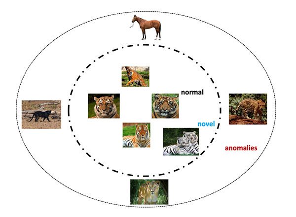
How can computer vision and deep learning detect natural disasters?

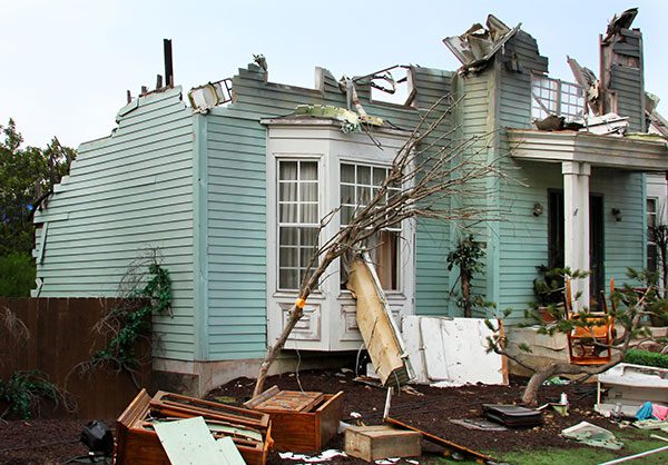
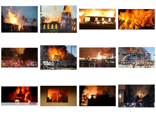
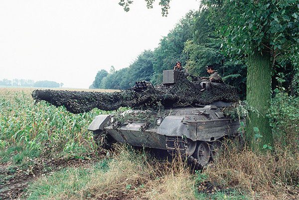
Figure 1: We can detect natural disasters with Keras and Deep Learning using a dataset of natural disaster images. (image source)

Natural disasters cannot be prevented — but they can be detected.

All around the world we use sensors to monitor for natural disasters:

• Seismic sensors (seismometers) and vibration sensors (seismoscopes) are used to monitor for earthquakes (and downstream tsunamis).
• Radar maps are used to detect the signature “hook echo” of a tornado (i.e., a hook that extends from the radar echo).
• Flood sensors are used to measure moisture levels while water level sensors monitor the height of water along a river, stream, etc.
• Wildfire sensors are still in their infancy but hopefully will be able to detect trace amounts of smoke and fire.

Each of these sensors is highly specialized to the task at hand — detect a natural disaster early, alert people, and allow them to get to safety.

Using computer vision we can augment existing sensors, thereby increasing the accuracy of natural disaster detectors, and most importantly, allow people to take precautions, stay safe, and prevent/reduce the number of deaths and injuries that happen due to these disasters.

Our natural disasters image dataset

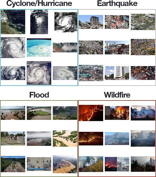
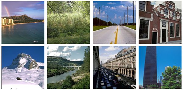
Figure 2: A dataset of natural disaster images. We’ll use this dataset to train a natural disaster detector with Keras and Deep Learning.

The dataset we are using here today was curated by PyImageSearch reader, Gautam Kumar.

Gautam used Google Images to gather a total of 4,428 images belonging to four separate classes:

• Cyclone/Hurricane: 928 images
• Earthquake: 1,350
• Flood: 1,073
• Wildfire: 1,077

He then trained a Convolutional Neural Network to recognize each of the natural disaster cases.

Gautam shared his work on his LinkedIn profile, gathering the attention of many deep learning practitioners (myself included). I asked him if he would be willing to (1) share his dataset with the PyImageSearch community and (2) allow me to write a tutorial using the dataset. Gautam agreed, and here we are today!

I again want to give a big, heartfelt thank you to Gautam for his hard work and contribution — be sure to thank him if you have the chance!

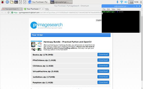
Downloading the natural disasters dataset

Figure 3: Gautam Kumar’s dataset for detecting natural disasters with Keras and deep learning.

You can use this link to download the original natural disasters dataset via Google Drive.

After you download the archive you should unzip it and inspect the contents:

$ tree --dirsfirst --filelimit 10 Cyclone_Wildfire_Flood_Earthquake_Database
Cyclone_Wildfire_Flood_Earthquake_Database
├── Cyclone [928 entries]
├── Earthquake [1350 entries]
├── Flood [1073 entries]
├── Wildfire [1077 entries]
└── readme.txt

4 directories, 1 file

Here you can see that each of the natural disasters has its own directory with examples of each class residing inside its respective parent directory.

Project structure

Using the

tree

$ tree --dirsfirst --filelimit 10
.
├── Cyclone_Wildfire_Flood_Earthquake_Database
│   ├── Cyclone [928 entries]
│   ├── Earthquake [1350 entries]
│   ├── Flood [1073 entries]
│   ├── Wildfire [1077 entries]
│   └── readme.txt
├── output
│   ├── natural_disaster.model
│   │   ├── assets
│   │   ├── variables
│   │   │   ├── variables.data-00000-of-00002
│   │   │   ├── variables.data-00001-of-00002
│   │   │   └── variables.index
│   │   └── saved_model.pb
│   ├── clr_plot.png
│   ├── lrfind_plot.png
│   └── training_plot.png
├── pyimagesearch
│   ├── __init__.py
│   ├── clr_callback.py
│   ├── config.py
│   └── learningratefinder.py
├── videos
│   ├── floods_101_nat_geo.mp4
│   ├── fort_mcmurray_wildfire.mp4
│   ├── hurricane_lorenzo.mp4
│   ├── san_andreas.mp4
│   └── terrific_natural_disasters_compilation.mp4
├── Cyclone_Wildfire_Flood_Earthquake_Database.zip
├── train.py
└── predict.py

11 directories, 20 files

Our project contains:

• The natural disaster dataset. Refer to the previous two sections.
• An

  output/

    directory where our model and plots will be stored. The results from my experiment are included.
• Our

  pyimagesearch

    module containing our Cyclical Learning Rate Keras callback, a configuration file, and Keras Learning Rate Finder.
• A selection of

  videos/

    for testing the video classification prediction script.
• Our training script,

  train.py

   . This script will perform fine-tuning on a VGG16 model pre-trained on the ImageNet dataset.
• Our video classification prediction script,

  predict.py

   , which performs a rolling average prediction to classify the video in real-time.

Our configuration file

Our project is going to span multiple Python files, so to keep our code tidy and organized (and ensure that we don’t have a multitude of command line arguments), let’s instead create a configuration file to store all important paths and variables.

Open up the

config.py

pyimagesearch

# import the necessary packages
import os

# initialize the path to the input directory containing our dataset
# of images
DATASET_PATH = "Cyclone_Wildfire_Flood_Earthquake_Database"

# initialize the class labels in the dataset
CLASSES = ["Cyclone", "Earthquake", "Flood", "Wildfire"]

The

os

Line 6 specifies the root path to our natural disaster dataset.

Line 7 provides the names of class labels (i.e. the names of the subdirectories in the dataset).

Let’s define our dataset splits:

# define the size of the training, validation (which comes from the
# train split), and testing splits, respectively
TRAIN_SPLIT = 0.75
VAL_SPLIT = 0.1
TEST_SPLIT = 0.25

Lines 13-15 house our training, testing, and validation split sizes. Take note that the validation split is 10% of the training split (not 10% of all the data).

Next, we’ll define our training parameters:

# define the minimum learning rate, maximum learning rate, batch size,
# step size, CLR method, and number of epochs
MIN_LR = 1e-6
MAX_LR = 1e-4
BATCH_SIZE = 32
STEP_SIZE = 8
CLR_METHOD = "triangular"
NUM_EPOCHS = 48

Lines 19 and 20 contain the minimum and maximum learning rate for Cyclical Learning Rates (CLR).We’ll learn how to set these learning rate values in the “Finding our initial learning rate” section below.

Lines 21-24 define the batch size, step size, CLR method, and the number of training epochs.

From there we’ll define the output paths:

# set the path to the serialized model after training
MODEL_PATH = os.path.sep.join(["output", "natural_disaster.model"])

# define the path to the output learning rate finder plot, training
# history plot and cyclical learning rate plot
LRFIND_PLOT_PATH = os.path.sep.join(["output", "lrfind_plot.png"])
TRAINING_PLOT_PATH = os.path.sep.join(["output", "training_plot.png"])
CLR_PLOT_PATH = os.path.sep.join(["output", "clr_plot.png"])

Lines 27-33 define the following output paths:

• Serialized model after training
• Learning rate finder plot
• Training history plot
• CLR plot

Implementing our training script with Keras

Our training procedure will consist of two steps:

1. Step #1: Use our learning rate finder to find optimal learning rates to fine-tune our VGG16 CNN on our dataset.
2. Step #2: Use our optimal learning rates in conjunction with Cyclical Learning Rates (CLR) to obtain a high accuracy model.

Our

train.py

Go ahead and open up

train.py

# set the matplotlib backend so figures can be saved in the background
import matplotlib
matplotlib.use("Agg")

# import the necessary packages
from tensorflow.keras.preprocessing.image import ImageDataGenerator
from tensorflow.keras.applications import VGG16
from tensorflow.keras.layers import Dropout
from tensorflow.keras.layers import Flatten
from tensorflow.keras.layers import Dense
from tensorflow.keras.layers import Input
from tensorflow.keras.models import Model
from tensorflow.keras.optimizers import SGD
from sklearn.preprocessing import LabelBinarizer
from sklearn.model_selection import train_test_split
from sklearn.metrics import classification_report
from pyimagesearch.learningratefinder import LearningRateFinder
from pyimagesearch.clr_callback import CyclicLR
from pyimagesearch import config
from imutils import paths
import matplotlib.pyplot as plt
import numpy as np
import argparse
import pickle
import cv2
import sys
import os

Lines 2-27 import necessary packages including:

• matplotlib

   : For plotting (using the

  "Agg"

    backend so plot images can be saved to disk).

• tensorflow

   : Imports including our

  VGG16

    CNN, data augmentation, layer types, and

  SGD

    optimizer.

• scikit-learn

   : Imports including a label binarizer, dataset splitting function, and an evaluation reporting tool.

• LearningRateFinder

   : Our Keras Learning Rate Finder class.

• CyclicLR

   : A Keras callback that oscillates learning rates, known as Cyclical Learning Rates. CLRs lead to faster convergence and typically require fewer experiments for hyperparameter updates.

• config

   : The custom configuration settings we reviewed in the previous section.

• paths

   : Includes a function for listing the image paths in a directory tree.

• cv2

   : OpenCV for preprocessing and display.

Let’s parse command line arguments and grab our image paths:

# construct the argument parser and parse the arguments
ap = argparse.ArgumentParser()
ap.add_argument("-f", "--lr-find", type=int, default=0,
	help="whether or not to find optimal learning rate")
args = vars(ap.parse_args())

# grab the paths to all images in our dataset directory and initialize
# our lists of images and class labels
print("[INFO] loading images...")
imagePaths = list(paths.list_images(config.DATASET_PATH))
data = []
labels = []

Recall that most of our settings are in

config.py

--lr-find

Line 38 grabs paths to all images in our dataset.

We then initialize two synchronized lists to hold our image 

data

labels

Let’s populate the

data

labels

# loop over the image paths
for imagePath in imagePaths:
	# extract the class label
	label = imagePath.split(os.path.sep)[-2]

	# load the image, convert it to RGB channel ordering, and resize
	# it to be a fixed 224x224 pixels, ignoring aspect ratio
	image = cv2.imread(imagePath)
	image = cv2.cvtColor(image, cv2.COLOR_BGR2RGB)
	image = cv2.resize(image, (224, 224))

	# update the data and labels lists, respectively
	data.append(image)
	labels.append(label)

# convert the data and labels to NumPy arrays
print("[INFO] processing data...")
data = np.array(data, dtype="float32")
labels = np.array(labels)
 
# perform one-hot encoding on the labels
lb = LabelBinarizer()
labels = lb.fit_transform(labels)

Lines 43-55 loop over

imagePaths

• Extracting the class

  label

    from the path (Line 45).
• Loading and preprocessing the

  image

    (Lines 49-51). Images are converted to RGB channel ordering and resized to 224×224 for VGG16.
• Adding the preprocessed

  image

    to the

  data

    list (Line 54).
• Adding the

  label

    to the

  labels

    list (Lines 55).

Line 59 performs a final preprocessing step by converting the

data

"float32"

Similarly, Line 60 converts

labels

From here, we’ll partition our data and set up data augmentation:

# partition the data into training and testing splits
(trainX, testX, trainY, testY) = train_test_split(data, labels,
	test_size=config.TEST_SPLIT, random_state=42)

# take the validation split from the training split
(trainX, valX, trainY, valY) = train_test_split(trainX, trainY,
	test_size=config.VAL_SPLIT, random_state=84)

# initialize the training data augmentation object
aug = ImageDataGenerator(
	rotation_range=30,
	zoom_range=0.15,
	width_shift_range=0.2,
	height_shift_range=0.2,
	shear_range=0.15,
	horizontal_flip=True,
	fill_mode="nearest")

Lines 67-72 construct training, testing, and validation splits.

Lines 75-82 instantiate our data augmentation object. Read more about data augmentation in my previous posts as well as in the Practitioner Bundle of Deep Learning for Computer Vision with Python.

At this point we’ll set up our VGG16 model for fine-tuning:

# load the VGG16 network, ensuring the head FC layer sets are left
# off
baseModel = VGG16(weights="imagenet", include_top=False,
	input_tensor=Input(shape=(224, 224, 3)))

# construct the head of the model that will be placed on top of the
# the base model
headModel = baseModel.output
headModel = Flatten(name="flatten")(headModel)
headModel = Dense(512, activation="relu")(headModel)
headModel = Dropout(0.5)(headModel)
headModel = Dense(len(config.CLASSES), activation="softmax")(headModel)

# place the head FC model on top of the base model (this will become
# the actual model we will train)
model = Model(inputs=baseModel.input, outputs=headModel)

# loop over all layers in the base model and freeze them so they will
# *not* be updated during the first training process
for layer in baseModel.layers:
	layer.trainable = False

# compile our model (this needs to be done after our setting our
# layers to being non-trainable
print("[INFO] compiling model...")
opt = SGD(lr=config.MIN_LR, momentum=0.9)
model.compile(loss="categorical_crossentropy", optimizer=opt,
	metrics=["accuracy"])

Lines 86 and 87 load

VGG16

Lines 91-95 create a new fully-connected layer head followed by Line 99 which adds the new FC layer to the body of VGG16.

Lines 103 and 104 mark the body of VGG16 as not trainable — we will be training (i.e. fine-tuning) only the FC layer head.

Lines 109-111 then

compile

SGD

The first time you run the script, you should set the

--lr-find

# check to see if we are attempting to find an optimal learning rate
# before training for the full number of epochs
if args["lr_find"] > 0:
	# initialize the learning rate finder and then train with learning
	# rates ranging from 1e-10 to 1e+1
	print("[INFO] finding learning rate...")
	lrf = LearningRateFinder(model)
	lrf.find(
		aug.flow(trainX, trainY, batch_size=config.BATCH_SIZE),
		1e-10, 1e+1,
		stepsPerEpoch=np.ceil((trainX.shape[0] / float(config.BATCH_SIZE))),
		epochs=20,
		batchSize=config.BATCH_SIZE)
 
	# plot the loss for the various learning rates and save the
	# resulting plot to disk
	lrf.plot_loss()
	plt.savefig(config.LRFIND_PLOT_PATH)
 
	# gracefully exit the script so we can adjust our learning rates
	# in the config and then train the network for our full set of
	# epochs
	print("[INFO] learning rate finder complete")
	print("[INFO] examine plot and adjust learning rates before training")
	sys.exit(0)

Line 115 checks to see if we should attempt to find optimal learning rates. Assuming so, we:

• Initialize

  LearningRateFinder

    (Line 119).
• Start training with a

  1e-10

    learning rate and exponentially increase it until we hit

  1e+1

    (Lines 120-125).
• Plot the loss vs. learning rate and save the resulting figure (Lines 129 and 130).
• Gracefully

  exit

    the script after printing a message instructing the user to inspect the learning rate finder plot (Lines 135-137).

After this code executes we now need to:

1. Step #1: Review the generated plot.
2. Step #2: Update

   config.py

   with our

   MIN_LR

     and

   MAX_LR

   , respectively.
3. Step #3: Train the network on our full dataset.

Assuming we have completed Steps #1 and #2, let’s now handle Step #3 where our minimum and maximum learning rate have already been found and updated in the config.

In this case, it is time to initialize our Cyclical Learning Rate class and commence training:

# otherwise, we have already defined a learning rate space to train
# over, so compute the step size and initialize the cyclic learning
# rate method
stepSize = config.STEP_SIZE * (trainX.shape[0] // config.BATCH_SIZE)
clr = CyclicLR(
	mode=config.CLR_METHOD,
	base_lr=config.MIN_LR,
	max_lr=config.MAX_LR,
	step_size=stepSize)

# train the network
print("[INFO] training network...")
H = model.fit_generator(
	aug.flow(trainX, trainY, batch_size=config.BATCH_SIZE),
	validation_data=(valX, valY),
	steps_per_epoch=trainX.shape[0] // config.BATCH_SIZE,
	epochs=config.NUM_EPOCHS,
	callbacks=[clr],
	verbose=1)

Lines 142-147 initialize our

CyclicLR

Lines 151-157 then train our

model

aug

clr

Upon training completion, we proceed to evaluate and save our

model

# evaluate the network and show a classification report
print("[INFO] evaluating network...")
predictions = model.predict(testX, batch_size=config.BATCH_SIZE)
print(classification_report(testY.argmax(axis=1),
	predictions.argmax(axis=1), target_names=config.CLASSES))

# serialize the model to disk
print("[INFO] serializing network to '{}'...".format(config.MODEL_PATH))
model.save(config.MODEL_PATH)

Line 161 makes predictions on our test set. Those predictions are passed into Lines 162 and 163 which print a classification report summary.

Line 167 serializes and saves the fine-tuned model to disk.

Finally, let’s plot both our training history and CLR history:

# construct a plot that plots and saves the training history
N = np.arange(0, config.NUM_EPOCHS)
plt.style.use("ggplot")
plt.figure()
plt.plot(N, H.history["loss"], label="train_loss")
plt.plot(N, H.history["val_loss"], label="val_loss")
plt.plot(N, H.history["accuracy"], label="train_acc")
plt.plot(N, H.history["val_accuracy"], label="val_acc")
plt.title("Training Loss and Accuracy")
plt.xlabel("Epoch #")
plt.ylabel("Loss/Accuracy")
plt.legend(loc="lower left")
plt.savefig(config.TRAINING_PLOT_PATH)

# plot the learning rate history
N = np.arange(0, len(clr.history["lr"]))
plt.figure()
plt.plot(N, clr.history["lr"])
plt.title("Cyclical Learning Rate (CLR)")
plt.xlabel("Training Iterations")
plt.ylabel("Learning Rate")
plt.savefig(config.CLR_PLOT_PATH)

Lines 170-181 generate a plot of our training history and save the plot to disk.

Note: In TensorFlow 2.0, the history dictionary keys have changed from

acc

accuracy

val_acc

val_accuracy

Lines 184-190 plot our Cyclical Learning Rate history and save the figure to disk.

Finding our initial learning rate

Before we attempt to fine-tune our model to recognize natural disasters, let’s first use our learning rate finder to find an optimal set of learning rate ranges. Using this optimal learning rate range we’ll then be able to apply Cyclical Learning Rates to improve our model accuracy.

Make sure you have both:

1. Used the “Downloads” section of this tutorial to download the source code.
2. Downloaded the dataset using the “Downloading the natural disasters dataset” section above.

From there, open up a terminal and execute the following command:

$ python train.py --lr-find 1
[INFO] loading images...
[INFO] processing data...
[INFO] compiling model...
[INFO] finding learning rate...
Epoch 1/20
94/94 [==============================] - 29s 314ms/step - loss: 9.7411 - accuracy: 0.2664
Epoch 2/20
94/94 [==============================] - 28s 295ms/step - loss: 9.5912 - accuracy: 0.2701
Epoch 3/20
94/94 [==============================] - 27s 291ms/step - loss: 9.4601 - accuracy: 0.2731
...
Epoch 12/20
94/94 [==============================] - 27s 290ms/step - loss: 2.7111 - accuracy: 0.7764
Epoch 13/20
94/94 [==============================] - 27s 286ms/step - loss: 5.9785 - accuracy: 0.6084
Epoch 14/20
47/94 [==============>...............] - ETA: 13s - loss: 10.8441 - accuracy: 0.3261
[INFO] learning rate finder complete
[INFO] examine plot and adjust learning rates before training

Provided the

train.py

lrfind_plot.png

Take a second now to inspect this image:

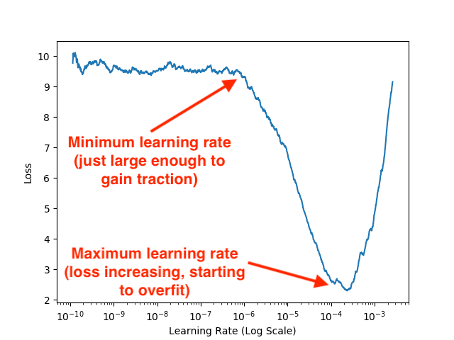
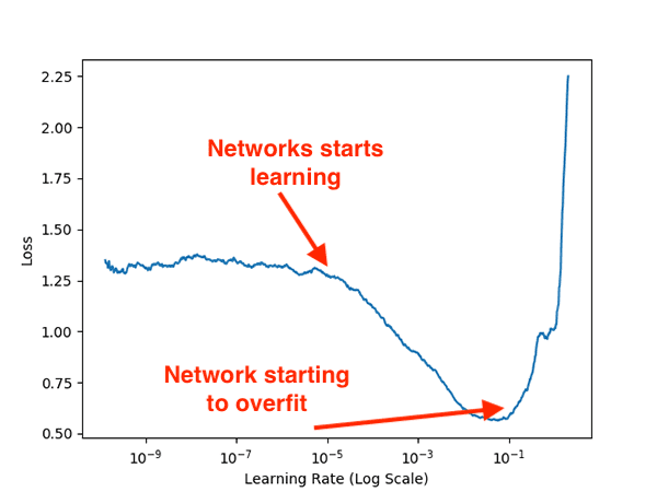
Figure 4: Using a Keras Learning Rate Finder to find the optimal learning rates to fine tune our CNN on our natural disaster dataset. We will use the dataset to train a model for detecting natural disasters with the Keras deep learning framework.

Examining the plot you can see that our model initially starts to learn and gain traction around

1e-6

Our loss continues to drop until approximately

1e-4

Our optimal learning rate range is, therefore,

1e-6

1e-4

Update our learning rates

Now that we know our optimal learning rates, let’s go back to our

config.py

# define the minimum learning rate, maximum learning rate, batch size,
# step size, CLR method, and number of epochs
MIN_LR = 1e-6
MAX_LR = 1e-4
BATCH_SIZE = 32
STEP_SIZE = 8
CLR_METHOD = "triangular"
NUM_EPOCHS = 48

Notice on Lines 19 and 20 (highlighted) of our configuration file that the

MIN_LR

MAX_LR

Training the natural disaster detection model with Keras

We can now fine-tune our model to recognize natural disasters!

Execute the following command which will train our network over the full set of epochs:

$ python train.py
[INFO] loading images...
[INFO] processing data...
[INFO] compiling model...
[INFO] training network...
Epoch 1/48
93/93 [==============================] - 32s 343ms/step - loss: 8.5819 - accuracy: 0.3254 - val_loss: 2.5915 - val_accuracy: 0.6829
Epoch 2/48
93/93 [==============================] - 30s 320ms/step - loss: 4.2144 - accuracy: 0.6194 - val_loss: 1.2390 - val_accuracy: 0.8573
Epoch 3/48
93/93 [==============================] - 29s 316ms/step - loss: 2.5044 - accuracy: 0.7605 - val_loss: 1.0052 - val_accuracy: 0.8862
Epoch 4/48
93/93 [==============================] - 30s 322ms/step - loss: 2.0702 - accuracy: 0.8011 - val_loss: 0.9150 - val_accuracy: 0.9070
Epoch 5/48
93/93 [==============================] - 29s 313ms/step - loss: 1.5996 - accuracy: 0.8366 - val_loss: 0.7397 - val_accuracy: 0.9268
...
Epoch 44/48
93/93 [==============================] - 28s 304ms/step - loss: 0.2180 - accuracy: 0.9275 - val_loss: 0.2608 - val_accuracy: 0.9476
Epoch 45/48
93/93 [==============================] - 29s 315ms/step - loss: 0.2521 - accuracy: 0.9178 - val_loss: 0.2693 - val_accuracy: 0.9449
Epoch 46/48
93/93 [==============================] - 29s 312ms/step - loss: 0.2330 - accuracy: 0.9284 - val_loss: 0.2687 - val_accuracy: 0.9467
Epoch 47/48
93/93 [==============================] - 29s 310ms/step - loss: 0.2120 - accuracy: 0.9322 - val_loss: 0.2646 - val_accuracy: 0.9476
Epoch 48/48
93/93 [==============================] - 29s 311ms/step - loss: 0.2237 - accuracy: 0.9318 - val_loss: 0.2664 - val_accuracy: 0.9485
[INFO] evaluating network...
              precision    recall  f1-score   support

     Cyclone       0.99      0.97      0.98       205
  Earthquake       0.96      0.93      0.95       362
       Flood       0.90      0.94      0.92       267
    Wildfire       0.96      0.97      0.96       273

    accuracy                           0.95      1107
   macro avg       0.95      0.95      0.95      1107
weighted avg       0.95      0.95      0.95      1107

[INFO] serializing network to 'output/natural_disaster.model'...

Here you can see that we are obtaining 95% accuracy when recognizing natural disasters in the testing set!

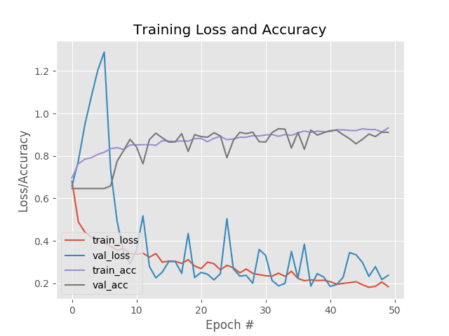
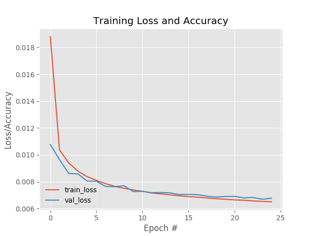
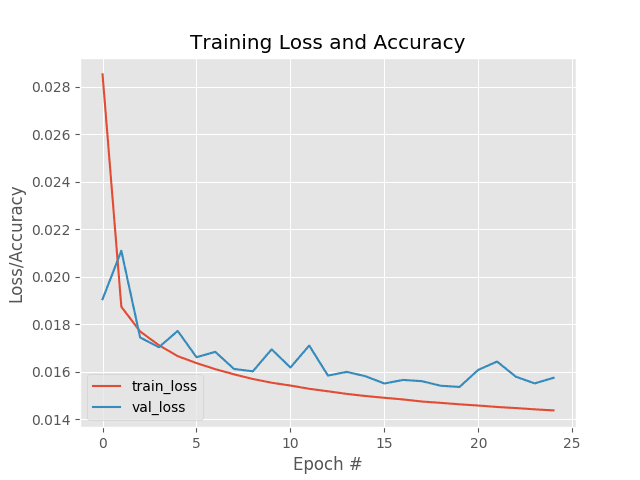
Examining our training plot we can see that our validation loss follows our training loss, implying there is little overfitting within our dataset itself:

Figure 5: Training history accuracy/loss curves for creating a natural disaster classifier using Keras and deep learning.

Finally, we have our learning rate plot which shows our our CLR callback oscillates the learning rate between our

MIN_LR

MAX_LR

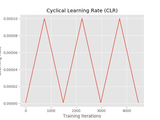
Figure 6: Cyclical learning rates are used with Keras and deep learning for detecting natural disasters.

Implementing our natural disaster prediction script

Now that our model has been trained, let’s see how we can use it to make predictions on images/video it has never seen before — and thereby pave the way for an automatic natural disaster detection system.

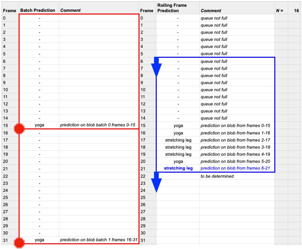
To create this script we’ll take advantage of the temporal nature of videos, specifically the assumption that subsequent frames in a video will have similar semantic contents.

By performing rolling prediction accuracy we’ll be able to “smooth out” the predictions and avoid “prediction flickering”.

I have already covered this near-identical script in-depth in my Video Classification with Keras and Deep Learning article. Be sure to refer to that article for the full background and more-detailed code explanations.

To accomplish natural disaster video classification let’s inspect

predict.py

# import the necessary packages
from tensorflow.keras.models import load_model
from pyimagesearch import config
from collections import deque
import numpy as np
import argparse
import cv2

# construct the argument parser and parse the arguments
ap = argparse.ArgumentParser()
ap.add_argument("-i", "--input", required=True,
	help="path to our input video")
ap.add_argument("-o", "--output", required=True,
	help="path to our output video")
ap.add_argument("-s", "--size", type=int, default=128,
	help="size of queue for averaging")
ap.add_argument("-d", "--display", type=int, default=-1,
	help="whether or not output frame should be displayed to screen")
args = vars(ap.parse_args())

Lines 2-7 load necessary packages and modules. In particular, we’ll be using

deque

collections

Lines 10-19 parse command line arguments including the path to our input/output videos, size of our rolling average queue, and whether we will display the output frame to our screen while the video is being generated.

Let’s go ahead and load our natural disaster classification model and initialize our queue + video stream:

# load the trained model from disk
print("[INFO] loading model and label binarizer...")
model = load_model(config.MODEL_PATH)

# initialize the predictions queue
Q = deque(maxlen=args["size"])

# initialize the video stream, pointer to output video file, and
# frame dimensions
print("[INFO] processing video...")
vs = cv2.VideoCapture(args["input"])
writer = None
(W, H) = (None, None)

With our

model

Q

vs

# loop over frames from the video file stream
while True:
	# read the next frame from the file
	(grabbed, frame) = vs.read()
 
	# if the frame was not grabbed, then we have reached the end
	# of the stream
	if not grabbed:
		break
 
	# if the frame dimensions are empty, grab them
	if W is None or H is None:
		(H, W) = frame.shape[:2]

	# clone the output frame, then convert it from BGR to RGB
	# ordering and resize the frame to a fixed 224x224
	output = frame.copy()
	frame = cv2.cvtColor(frame, cv2.COLOR_BGR2RGB)
	frame = cv2.resize(frame, (224, 224))
	frame = frame.astype("float32")

Lines 38-47 grab a

frame

Lines 51-54 duplicate our

frame

output

Now let’s make a natural disaster prediction on the frame:

# make predictions on the frame and then update the predictions
	# queue
	preds = model.predict(np.expand_dims(frame, axis=0))[0]
	Q.append(preds)

	# perform prediction averaging over the current history of
	# previous predictions
	results = np.array(Q).mean(axis=0)
	i = np.argmax(results)
	label = config.CLASSES[i]

Lines 58 and 59 perform inference and add the predictions to our queue.

Line 63 performs a rolling average prediction of the predictions available in the

Q

Lines 64 and 65 then extract the highest probability class label so that we can annotate our frame:

# draw the activity on the output frame
	text = "activity: {}".format(label)
	cv2.putText(output, text, (35, 50), cv2.FONT_HERSHEY_SIMPLEX,
		1.25, (0, 255, 0), 5)
 
	# check if the video writer is None
	if writer is None:
		# initialize our video writer
		fourcc = cv2.VideoWriter_fourcc(*"MJPG")
		writer = cv2.VideoWriter(args["output"], fourcc, 30,
			(W, H), True)
 
	# write the output frame to disk
	writer.write(output)
 
	# check to see if we should display the output frame to our
	# screen
	if args["display"] > 0:
		# show the output image
		cv2.imshow("Output", output)
		key = cv2.waitKey(1) & 0xFF
	 
		# if the `q` key was pressed, break from the loop
		if key == ord("q"):
			break
 
# release the file pointers
print("[INFO] cleaning up...")
writer.release()
vs.release()

Lines 68-70 annotate the natural disaster activity in the corner of the

output

Lines 73-80 handle writing the

output

If the

--display

Otherwise, processing continues until completion at which point the loop is finished and we perform cleanup (Lines 95 and 96).

Predicting natural disasters with Keras

For the purposes of this tutorial, I downloaded example natural disaster videos via YouTube — the exact videos are listed in the “Credits” section below. You can either use your own example videos or download the videos via the credits list.

Either way, make sure you have used the “Downloads” section of this tutorial to download the source code and pre-trained natural disaster prediction model.

Once downloaded you can use the following command to launch the

predict.py

$ python predict.py --input videos/terrific_natural_disasters_compilation.mp4 \
	--output output/natural_disasters_output.avi
[INFO] processing video...
[INFO] cleaning up...

Here you can see a sample result of our model correctly classifying this video clip as “flood”:

Figure 7: Natural disaster “flood” classification with Keras and Deep Learning.

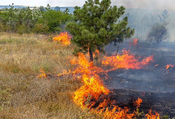
The following example comes from the 2016 Fort McMurray wildfire:

Figure 8: Detecting “wildfires” and other natural disasters with Keras, deep learning, and computer vision.

For fun, I then tried applying the natural disaster detector to the movie San Andreas (2015):

Figure 9: Detecting “earthquake” damage with Keras, deep learning, and Python.

Notice how our model was able to correctly label the video clip as an (overly dramatized) earthquake.

You can find a full demo video below:

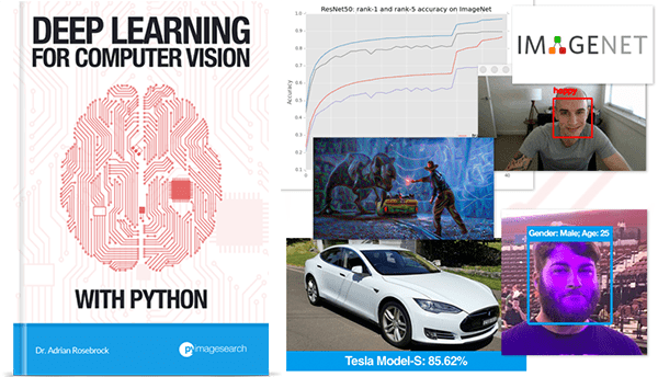
Where to next?

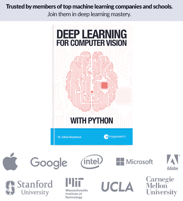
Figure 10: My deep learning book is the go-to resource for deep learning students, developers, researchers, and hobbyists, alike. Use the book to build your skillset from the bottom up, or read it to gain a deeper understanding. Don’t be left in the dust as the fast paced AI revolution continues to accelerate.

Today’s tutorial helped us solve a real-world classification problem for classifying natural disaster videos.

Such an application could be:

• Deployed along riverbeds and streams to monitor water levels and detect floods early.
• Utilized by park rangers to monitor for wildfires.
• Employed by meteorologists to automatically detect hurricanes/cyclones.
• Used by television news companies to sort their archives of video footage.

We created our natural disaster detector by utilizing a number of important deep learning techniques:

• Fine-tuning a Convolutional Neural Network that was trained on ImageNet
• Using a Keras Learning Rate Finder
• Implementing the Cyclical Learning Rate callback into our training process to improve model accuracy
• Performing video classification with a rolling frame classification average approach

Admittedly, these are advanced concepts in the realm of deep learning and computer vision. If you have your own real-world project you’re trying to solve, you need a strong deep learning foundation in addition to familiarity with advanced concepts.

To jumpstart your education, including discovering my tips, suggestions, and best practices when training deep neural networks, be sure to refer to my book, Deep Learning for Computer Vision with Python.

Inside the book I cover:

1. Deep learning fundamentals and theory without unnecessary mathematical fluff. I present the basic equations and back them up with code walkthroughs that you can implement and easily understand. You don’t need a degree in advanced mathematics to understand this book.
2. More details on learning rates, tuning them, and how a solid understanding of the concept dramatically impacts the accuracy of your model.
3. How to spot underfitting and overfitting on-the-fly, saving you days of training time.
4. How to perform fine-tuning on pre-trained models, which is often the place I start to obtain a baseline result to beat.
5. My tips/tricks, suggestions, and best practices for training CNNs.

To learn more about the book, and grab the table of contents + free sample chapters, just click here!

Credits

Dataset curator:

• Gautam Kumar

Video sources for the demo:

• Hurricane Lorenzo Wreaks Havoc on The Azores on its way to UK
• Fort McMurray wildfire: A timeline of a disaster
• Floods 101 | National Geographic
• 9.6 Magnitude Earthquake (Scenes from the film San Andreas 2015)
• Terrific National Disasters Compilation

Audio for the demo video:

• Bensound’s “Epic”

Summary

In this tutorial, you learned how to use computer vision and the Keras deep learning library to automatically detect natural disasters from images.

To create our natural disaster detector we fine-tuned VGG16 (pre-trained on ImageNet) on a dataset of 4,428 images belonging to four classes:

• Cyclone/hurricane
• Earthquake
• Flood
• Wildfire

After our model was trained we evaluated it on the testing set, finding that it obtained 95% classification accuracy.

Using this model you can continue to perform research in natural disaster detection, ultimately helping save lives and reduce injury.

I hope you enjoyed this post!

To download the source code to the post (and be notified when future tutorials are published on PyImageSearch), just enter your email address in the form below.

Downloads:

If you would like to download the code and images used in this post, please enter your email address in the form below. Not only will you get a .zip of the code, I’ll also send you a FREE 17-page Resource Guide on Computer Vision, OpenCV, and Deep Learning. Inside you'll find my hand-picked tutorials, books, courses, and libraries to help you master CV and DL! Sound good? If so, enter your email address and I’ll send you the code immediately!

Email address:

Website

The post Detecting Natural Disasters with Keras and Deep Learning appeared first on PyImageSearch.

In this tutorial, you will learn how to detect fire and smoke using Computer Vision, OpenCV, and the Keras Deep Learning library.

Today’s tutorial is inspired by an email I received last week from PyImageSearch reader, Daniel.

Daniel writes:

Hey Adrian, I’m not sure if you’ve seen the news, but my home state of California has been absolutely ravaged by wildfires over the past few weeks.

My family lives in the Los Angeles area, not too far from the Getty fire. It’s hard not to be concerned about our home and our safety.

It’s a scary situation and it got me thinking:

Do you think computer vision could be used to detect wildfires? What about fires that start in people’s homes?

If you could write a tutorial on the topic I would appreciate it. I’d love to learn from it and do my part to help others.

The short answer is, yes, computer vision and deep learning can be used to detect wildfires:

• IoT/Edge devices equipped with cameras can be deployed strategically throughout hillsides, ridges, and high elevation areas, automatically monitoring for signs of smoke or fire.
• Drones and quadcopters can be flown above areas prone to wildfires, strategically scanning for smoke.
• Satellites can be used to take photos of large acreage areas while computer vision and deep learning algorithms process these images, looking for signs of smoke.

That’s all fine and good for wildfires — but what if you wanted to monitor your own home for smoke or fire?

The answer there is to augment existing sensors to aid in fire/smoke detection:

• Existing smoke detectors utilize photoelectric sensors and a light source to detect if the light source particles are being scattered (implying smoke is present).
• You could then distribute temperature sensors around the house to monitor the temperature of each room.
• Cameras could also be placed in areas where fires are likely to start (kitchen, garage, etc.).
• Each individual sensor could be used to trigger an alarm or you could relay the sensor information to a central hub that aggregates and analyzes the sensor data, computing a probability of a home fire.

Unfortunately, that’s all easier said than done.

While there are 100s of computer vision/deep learning practitioners around the world actively working on fire and smoke detection (including PyImageSearch Gurus member, David Bonn), it’s still an open-ended problem.

That said, today I’ll help you get your start in smoke and fire detection — by the end of this tutorial, you’ll have a deep learning model capable of detecting fire in images (I’ve even included my pre-trained model to get you up and running immediately).

To learn how to create your own fire and smoke detector with Computer Vision, Deep Learning, and Keras, just keep reading!

Fire and smoke detection with Keras and Deep Learning

Figure 1: Wildfires can quickly become out of control and endanger lives in many parts of the world. In this article, we will learn to conduct fire and smoke detection with Keras and deep learning.

In the first part of this tutorial we’ll discuss the two datasets we’ll be using for fire and smoke detection.

From there we’ll review or directory structure for the project and then implement

FireDetectionNet

Next, we’ll train our fire detection model and analyze the classification accuracy and results.

We’ll wrap up the tutorial by discussing some of the limitations and drawbacks of the approach, including how you can improve and extend the method.

Our fire and smoke dataset

Figure 2: Today’s fire detection dataset is curated by Gautam Kumar and pruned by David Bonn (both of whom are PyImageSearch readers). We will put the dataset to work with Keras and deep learning to create a fire/smoke detector.

The dataset we’ll be using for fire and smoke examples was curated by PyImageSearch reader, Gautam Kumar.

Guatam gathered a total of 1,315 images by searching Google Images for queries related to the term “fire”, “smoke”, etc.

However, the original dataset has not been cleansed of extraneous, irrelevant images that are not related to fire and smoke (i.e., examples of famous buildings before a fire occurred).

Fellow PyImageSearch reader, David Bonn, took the time to manually go through the fire/smoke images and identify ones that should not be included.

Note: I took the list of extraneous images identified by David and then created a shell script to delete them from the dataset. The shell script can be found in the “Downloads” section of this tutorial.

The 8-scenes dataset

Figure 3: We will combine Gautam’s fire dataset with the 8-scenes natural image dataset so that we can classify Fire vs. Non-fire using Keras and deep learning.

The dataset we’ll be using for Non-fire examples is called 8-scenes as it contains 2,688 image examples belonging to eight natural scene categories (all without fire):

1. Coast
2. Mountain
3. Forest
4. Open country
5. Street
6. Inside city
7. Tall buildings
8. Highways

The dataset was originally curated by Oliva and Torralba in their 2001 paper, Modeling the shape of the scene: a holistic representation of the spatial envelope.

The 8-scenes dataset is a natural complement to our fire/smoke dataset as it depicts natural scenes as they should look without fire or smoke present.

While this dataset has 8 unique classes, we will consider the dataset as a single Non-fire class when we combine it with Gautam’s Fire dataset.

Project structure

Figure 4: The project structure for today’s tutorial on fire and smoke detection with deep learning using the Keras/TensorFlow framework.

Go ahead and grab today’s .zip from the source code and pre-trained model using the “Downloads” section of this blog post.

From there you can unzip it on your machine and your project will look like Figure 4. There is an exception: neither dataset .zip (white arrows) will be present yet. We will download, extract, and prune the datasets in the next section.

Our

output/

• Our serialized fire detection model. We will train the model today with Keras and deep learning.
• The Learning Rate Finder plot will be generated and inspected for the optimal learning rate prior to training.
• A training history plot will be generated upon completion of the training process.
• The 

  examples/

    subdirectory will be populated by

  predict_fire.py

    with sample images that will be annotated for demonstration and verification purposes.

Our

pyimagesearch

• config.py

   : Our customizable configuration.

• FireDetectionNet

   : Our Keras Convolutional Neural Network class designed specifically for detecting fire and smoke.

• LearningRateFinder

   : A Keras class for assisting in the process of finding the optimal learning rate for deep learning training.

The root of the project contains three scripts:

• prune.sh

   : A simple bash script that removes irrelevant images from Gautam’s fire dataset.

• train.py

   : Our Keras deep learning training script. This script has two modes of operation: (1) Learning Rate Finder mode,and (2) training mode.

• predict_fire.py

   : A quick and dirty script which samples images from our dataset, generating annotated Fire/Non-fire images for verification.

Let’s move on to preparing our Fire/Non-fire dataset in the next section.

Preparing our Fire and Non-fire combined dataset

Preparing our Fire and Non-fire dataset involves a four-step process:

1. Step #1: Ensure you followed the instructions in the previous section to grab and unzip today’s files from the “Downloads” section.
2. Step #2: Download and extract the fire/smoke dataset into the project.
3. Step #3: Prune the fire/smoke dataset for extraneous, irrelevant files.
4. Step #4: Download and extract the 8-scenes dataset into the project.

The result of Steps #2-4 will be a dataset consisting of two classes:

• Fire
• Non-fire

Combining datasets is a tactic I often use. It saves valuable time and often leads to a great model.

Let’s begin putting our combined dataset together.

Step #2: Download and extract the fire/smoke dataset into the project.

Download the fire/smoke dataset using this link. Store the .zip in the

keras-fire-detection/

Once downloaded, unzip the dataset:

$ unzip Robbery_Accident_Fire_Database2.zip

Step #3: Prune the dataset for extraneous, irrelevant files.

Execute the

prune.sh

$ sh prune.sh

At this point, we have Fire data. Now we need Non-fire data for our two-class problem.

Step #4: Download and extract the 8-scenes dataset into the project.

Download the 8-scenes dataset using this link. Store the .zip in the

keras-fire-detection/

Once downloaded, navigate to the project folder and unarchive the dataset:

$ unzip spatial_envelope_256x256_static_8outdoorcategories.zip

Review Project + Dataset Structure

At this point, it is time to inspect our directory structure once more. Yours should be identical to mine:

$ tree --dirsfirst --filelimit 10
.
├── Robbery_Accident_Fire_Database2
│   ├── Accident [887 entries]
│   ├── Fire [1315 entries]
│   ├── Robbery [2073 entries]
│   └── readme.txt
├── spatial_envelope_256x256_static_8outdoorcategories [2689 entries]
├── output
│   ├── examples [48 entries]
│   ├── fire_detection.model
│   │   ├── assets
│   │   ├── variables
│   │   │   ├── variables.data-00000-of-00002
│   │   │   ├── variables.data-00001-of-00002
│   │   │   └── variables.index
│   │   └── saved_model.pb
│   ├── lrfind_plot.png
│   └── training_plot.png
├── pyimagesearch
│   ├── __init__.py
│   ├── config.py
│   ├── firedetectionnet.py
│   └── learningratefinder.py
├── Robbery_Accident_Fire_Database.zip
├── spatial_envelope_256x256_static_8outdoorcategories.zip
├── prune.sh
├── train.py
└── predict_fire.py

11 directories, 16 files

Ensure your dataset is pruned (i.e. the

Fire/

Our configuration file

This project will span multiple Python files that will need to be executed, so let’s store all important variables in a single

config.py

Open up

config.py

# import the necessary packages
import os

# initialize the path to the fire and non-fire dataset directories
FIRE_PATH = os.path.sep.join(["Robbery_Accident_Fire_Database2",
	"Fire"])
NON_FIRE_PATH = "spatial_envelope_256x256_static_8outdoorcategories"

# initialize the class labels in the dataset
CLASSES = ["Non-Fire", "Fire"]

We’ll use the

os

Lines 5-7 contain paths to our (1) Fire images, and (2) Non-fire images.

Line 10 is a list of our two class names.

Let’s set a handful of training parameters:

# define the size of the training and testing split
TRAIN_SPLIT = 0.75
TEST_SPLIT = 0.25

# define the initial learning rate, batch size, and number of epochs
INIT_LR = 1e-2
BATCH_SIZE = 64
NUM_EPOCHS = 50

Lines 13 and 14 define the size of our training and testing dataset splits.

Lines 17-19 contain three hyperparameters — the initial learning rate, batch size, and number of epochs to train for.

From here, we’ll define a few paths:

# set the path to the serialized model after training
MODEL_PATH = os.path.sep.join(["output", "fire_detection.model"])

# define the path to the output learning rate finder plot and
# training history plot
LRFIND_PLOT_PATH = os.path.sep.join(["output", "lrfind_plot.png"])
TRAINING_PLOT_PATH = os.path.sep.join(["output", "training_plot.png"])

Lines 22-27 include paths to:

• Our yet-to-be-trained serialized fire detection model.
• The Learning Rate Finder plot which we will analyze to set our initial learning rate.
• A training accuracy/loss history plot.

To wrap up our config we’ll define settings for prediction spot-checking:

# define the path to the output directory that will store our final
# output with labels/annotations along with the number of images to
# sample
OUTPUT_IMAGE_PATH = os.path.sep.join(["output", "examples"])
SAMPLE_SIZE = 50

Our prediction script will sample and annotate images using our model.

Lines 32 and 33 include the path to output directory where we’ll store output classification results and the number of images to sample.

Implementing our fire detection Convolutional Neural Network

Figure 5: FireDetectionNet is a deep learning fire/smoke classification network built with the Keras deep learning framework.

In this section we’ll implement

FireDetectionNet

This network utilizes depthwise separable convolution rather than standard convolution as depthwise separable convolution:

• Is more efficient, as Edge/IoT devices will have limited CPU and power draw.
• Requires less memory, as again, Edge/IoT devices have limited RAM.
• Requires less computation, as we have limited CPU horsepower.
• Can perform better than standard convolution in some cases, which can lead to a better fire/smoke detector.

Let’s get started implementing

FireDetectioNet

firedetectionnet.py

# import the necessary packages
from tensorflow.keras.models import Sequential
from tensorflow.keras.layers import BatchNormalization
from tensorflow.keras.layers import SeparableConv2D
from tensorflow.keras.layers import MaxPooling2D
from tensorflow.keras.layers import Activation
from tensorflow.keras.layers import Flatten
from tensorflow.keras.layers import Dropout
from tensorflow.keras.layers import Dense

class FireDetectionNet:
	@staticmethod
	def build(width, height, depth, classes):
		# initialize the model along with the input shape to be
		# "channels last" and the channels dimension itself
		model = Sequential()
		inputShape = (height, width, depth)
		chanDim = -1

Our TensorFlow 2.0 Keras imports span from Lines 2-9. We will use Keras’ Sequential API to build our fire detection CNN.

Line 11 defines our

FireDetectionNet

build

The

build

width

height

depth

classes

We then initialize the

model

inputShape

From here we’ll define our first set of

CONV => RELU => POOL

# CONV => RELU => POOL
		model.add(SeparableConv2D(16, (7, 7), padding="same",
			input_shape=inputShape))
		model.add(Activation("relu"))
		model.add(BatchNormalization(axis=chanDim))
		model.add(MaxPooling2D(pool_size=(2, 2)))

These layers use a larger kernel size to both (1) reduce the input volume spatial dimensions faster, and (2) detect larger color blobs that contain fire.

We’ll then define more

CONV => RELU => POOL

# CONV => RELU => POOL
		model.add(SeparableConv2D(32, (3, 3), padding="same"))
		model.add(Activation("relu"))
		model.add(BatchNormalization(axis=chanDim))
		model.add(MaxPooling2D(pool_size=(2, 2)))

		# (CONV => RELU) * 2 => POOL
		model.add(SeparableConv2D(64, (3, 3), padding="same"))
		model.add(Activation("relu"))
		model.add(BatchNormalization(axis=chanDim))
		model.add(SeparableConv2D(64, (3, 3), padding="same"))
		model.add(Activation("relu"))
		model.add(BatchNormalization(axis=chanDim))
		model.add(MaxPooling2D(pool_size=(2, 2)))

Lines 34-40 allow our model to learn richer features by stacking two sets of

CONV => RELU

POOL

From here we’ll create our fully-connected head of the network:

# first set of FC => RELU layers
		model.add(Flatten())
		model.add(Dense(128))
		model.add(Activation("relu"))
		model.add(BatchNormalization())
		model.add(Dropout(0.5))

		# second set of FC => RELU layers
		model.add(Dense(128))
		model.add(Activation("relu"))
		model.add(BatchNormalization())
		model.add(Dropout(0.5))

		# softmax classifier
		model.add(Dense(classes))
		model.add(Activation("softmax"))

		# return the constructed network architecture
		return model

Lines 43-53 add two sets of

FC => RELU

Lines 56 and 57 append our Softmax classifier prior to Line 60 returning the

model

Creating our training script

Our training script will be responsible for:

1. Loading our Fire and Non-fire combined dataset from disk.
2. Instantiating our

   FireDetectionNet

   architecture.
3. Finding our optimal learning rate by using our

   LearningRateFinder

   class.
4. Taking the optimal learning rate and training our network for the full set of epochs.

Let’s get started!

Open up the

train.py

# set the matplotlib backend so figures can be saved in the background
import matplotlib
matplotlib.use("Agg")

# import the necessary packages
from tensorflow.keras.preprocessing.image import ImageDataGenerator
from tensorflow.keras.optimizers import SGD
from tensorflow.keras.utils import to_categorical
from sklearn.model_selection import train_test_split
from sklearn.metrics import classification_report
from pyimagesearch.learningratefinder import LearningRateFinder
from pyimagesearch.firedetectionnet import FireDetectionNet
from pyimagesearch import config
from imutils import paths
import matplotlib.pyplot as plt
import numpy as np
import argparse
import cv2
import sys

Lines 1-19 handle our imports:

• matplotlib

   : For generating plots with Python. Line 3 sets the backend so we can save our plots as image files.

• tensorflow.keras

   : Our TensorFlow 2.0 imports including data augmentation, stochastic gradient descent optimizer, and one-hot label encoder.

• sklearn

   : Two imports for dataset splitting and classification reporting.

• LearningRateFinder

   : A class we will use for finding an optimal learning rate prior to training. When we operate our script in this mode, it will generate a plot for us to (1) manually inspect and (2) insert the optimal learning rate into our configuration file.

• FireDetectionNet

   : The fire/smoke Convolutional Neural Network (CNN) that we built in the previous section.

• config

   : Our configuration file of settings for this training script (it also contains settings for our prediction script).

• paths

   : Contains functions from my imutils package to list images in a directory tree.

• argparse

   : For parsing command line argument flags.

• cv2

   : OpenCV is used for loading and preprocessing images.

Now that we’ve imported packages, let’s define a reusable function to load our dataset:

def load_dataset(datasetPath):
	# grab the paths to all images in our dataset directory, then
	# initialize our lists of images
	imagePaths = list(paths.list_images(datasetPath))
	data = []

	# loop over the image paths
	for imagePath in imagePaths:
		# load the image and resize it to be a fixed 128x128 pixels,
		# ignoring aspect ratio
		image = cv2.imread(imagePath)
		image = cv2.resize(image, (128, 128))

		# add the image to the data lists
		data.append(image)

	# return the data list as a NumPy array
	return np.array(data, dtype="float32")

Our

load_dataset

Line 21 defines the function which accepts a path to the dataset.

Line 24 grabs all image paths in the dataset.

Lines 28-35 loop over the

imagePaths

data

Line 38 returns the

data

We’ll now parse a single command line argument:

# construct the argument parser and parse the arguments
ap = argparse.ArgumentParser()
ap.add_argument("-f", "--lr-find", type=int, default=0,
	help="whether or not to find optimal learning rate")
args = vars(ap.parse_args())

The

--lr-find

1

--lr-find

Let’s go ahead and load our

data

# load the fire and non-fire images
print("[INFO] loading data...")
fireData = load_dataset(config.FIRE_PATH)
nonFireData = load_dataset(config.NON_FIRE_PATH)

# construct the class labels for the data
fireLabels = np.ones((fireData.shape[0],))
nonFireLabels = np.zeros((nonFireData.shape[0],))

# stack the fire data with the non-fire data, then scale the data
# to the range [0, 1]
data = np.vstack([fireData, nonFireData])
labels = np.hstack([fireLabels, nonFireLabels])
data /= 255

Lines 48 and 49 load and resize the Fire and Non-fire images.

Lines 52 and 53 construct labels for both classes (

1

0

Subsequently, we stack the

data

labels

Line 59 scales pixel intensities to the range [0, 1].

We have three more steps to prepare our data:

# perform one-hot encoding on the labels and account for skew in the
# labeled data
labels = to_categorical(labels, num_classes=2)
classTotals = labels.sum(axis=0)
classWeight = classTotals.max() / classTotals

# construct the training and testing split
(trainX, testX, trainY, testY) = train_test_split(data, labels,
	test_size=config.TEST_SPLIT, random_state=42)

First, we perform one-hot encoding on our

labels

Then, we account for skew in our dataset (Lines 64 and 65). To do so, we compute the

classWeight

Lines 68 and 69 construct training and testing splits based on our config (in my config I have the split set to 75% training/25% testing).

Next, we’ll initialize data augmentation and compile our

FireDetectionNet

# initialize the training data augmentation object
aug = ImageDataGenerator(
	rotation_range=30,
	zoom_range=0.15,
	width_shift_range=0.2,
	height_shift_range=0.2,
	shear_range=0.15,
	horizontal_flip=True,
	fill_mode="nearest")

# initialize the optimizer and model
print("[INFO] compiling model...")
opt = SGD(lr=config.INIT_LR, momentum=0.9,
	decay=config.INIT_LR / config.NUM_EPOCHS)
model = FireDetectionNet.build(width=128, height=128, depth=3,
	classes=2)
model.compile(loss="binary_crossentropy", optimizer=opt,
	metrics=["accuracy"])

Lines 74-79 instantiate our data augmentation object.

We then

build

compile

FireDetectionNet

SGD

Let’s handle our Learning Rate Finder mode:

# check to see if we are attempting to find an optimal learning rate
# before training for the full number of epochs
if args["lr_find"] > 0:
	# initialize the learning rate finder and then train with learning
	# rates ranging from 1e-10 to 1e+1
	print("[INFO] finding learning rate...")
	lrf = LearningRateFinder(model)
	lrf.find(
		aug.flow(trainX, trainY, batch_size=config.BATCH_SIZE),
		1e-10, 1e+1,
		stepsPerEpoch=np.ceil((trainX.shape[0] / float(config.BATCH_SIZE))),
		epochs=20,
		batchSize=config.BATCH_SIZE,
		classWeight=classWeight)

	# plot the loss for the various learning rates and save the
	# resulting plot to disk
	lrf.plot_loss()
	plt.savefig(config.LRFIND_PLOT_PATH)

	# gracefully exit the script so we can adjust our learning rates
	# in the config and then train the network for our full set of
	# epochs
	print("[INFO] learning rate finder complete")
	print("[INFO] examine plot and adjust learning rates before training")
	sys.exit(0)

Line 92 checks to see if we should attempt to find optimal learning rates. Assuming so, we:

• Initialize

  LearningRateFinder

    (Line 96).
• Start training with a

  1e-10

    learning rate and exponentially increase it until we hit

  1e+1

    (Lines 97-103).
• Plot the loss vs. learning rate and save the resulting figure (Lines 107 and 108).
• Gracefully

  exit

    the script after printing a couple of messages to the user (Lines 115).

After this code executes we now need to:

1. Step #1: Manually inspect the generated learning rate plot.
2. Step #2: Update

   config.py

   with our

   INIT_LR

    (i.e., the optimal learning rate we determined by analyzing the plot).
3. Step #3: Train the network on our full dataset.

Assuming we have completed Step #1 and Step #2, now let’s handle the Step #3 where our initial learning rate has been determined and updated in the config. In this case, it is time to handle training mode in our script:

# train the network
print("[INFO] training network...")
H = model.fit_generator(
	aug.flow(trainX, trainY, batch_size=config.BATCH_SIZE),
	validation_data=(testX, testY),
	steps_per_epoch=trainX.shape[0] // config.BATCH_SIZE,
	epochs=config.NUM_EPOCHS,
	class_weight=classWeight,
	verbose=1)

Lines 119-125 train our fire detection

model

Finally, we’ll evaluate the model, serialize it to disk, and plot the training history:

# evaluate the network and show a classification report
print("[INFO] evaluating network...")
predictions = model.predict(testX, batch_size=config.BATCH_SIZE)
print(classification_report(testY.argmax(axis=1),
	predictions.argmax(axis=1), target_names=config.CLASSES))

# serialize the model to disk
print("[INFO] serializing network to '{}'...".format(config.MODEL_PATH))
model.save(config.MODEL_PATH)

# construct a plot that plots and saves the training history
N = np.arange(0, config.NUM_EPOCHS)
plt.style.use("ggplot")
plt.figure()
plt.plot(N, H.history["loss"], label="train_loss")
plt.plot(N, H.history["val_loss"], label="val_loss")
plt.plot(N, H.history["accuracy"], label="train_acc")
plt.plot(N, H.history["val_accuracy"], label="val_acc")
plt.title("Training Loss and Accuracy")
plt.xlabel("Epoch #")
plt.ylabel("Loss/Accuracy")
plt.legend(loc="lower left")
plt.savefig(config.TRAINING_PLOT_PATH)

Lines 129-131 make predictions on test data and print a classification report in our terminal.

Line 135 serializes the

model

Lines 138-149 generate a historical plot of accuracy/loss curves during training. We will inspect this plot for overfitting or underfitting.

Training the fire detection model with Keras

Training our fire detection model is broken down into three steps:

1. Step #1: Run the

   train.py

   script with the

   --lr-find

   command line argument to find our optimal learning rate.
2. Step #2: Update Line 17 of our configuration file (

   config.py

    ) to set our

   INIT_LR

   value as the optimal learning rate.
3. Step #3: Execute the

   train.py

   script again, but this time let it train for the full set of epochs.

Start by using the “Downloads” section of this tutorial to download the source code to this tutorial.

From there you can perform Step #1 by executing the following command:

$ python train.py --lr-find 1
[INFO] loading data...
[INFO] finding learning rate...
Epoch 1/20
47/47 [==============================] - 10s 221ms/step - loss: 1.2949 - accuracy: 0.4923
Epoch 2/20
47/47 [==============================] - 11s 228ms/step - loss: 1.3315 - accuracy: 0.4897
Epoch 3/20
47/47 [==============================] - 10s 218ms/step - loss: 1.3409 - accuracy: 0.4860
Epoch 4/20
47/47 [==============================] - 10s 215ms/step - loss: 1.3973 - accuracy: 0.4770
Epoch 5/20
47/47 [==============================] - 10s 219ms/step - loss: 1.3170 - accuracy: 0.4957
...
Epoch 15/20
47/47 [==============================] - 10s 216ms/step - loss: 0.5097 - accuracy: 0.7728
Epoch 16/20
47/47 [==============================] - 10s 217ms/step - loss: 0.5507 - accuracy: 0.7345
Epoch 17/20
47/47 [==============================] - 10s 220ms/step - loss: 0.7554 - accuracy: 0.7089
Epoch 18/20
47/47 [==============================] - 10s 220ms/step - loss: 1.1833 - accuracy: 0.6606
Epoch 19/20
37/47 [======================>.......] - ETA: 2s - loss: 3.1446 - accuracy: 0.6338
[INFO] learning rate finder complete
[INFO] examine plot and adjust learning rates before training

Figure 6: Analyzing our optimal deep learning rate finder plot. We will use the optimal learning rate to train a fire/smoke detector using Keras and Python.

Examining Figure 6 above you can see that our network is able to gain traction and start to learn around

1e-5

The lowest loss can be found between

1e-2

1e-1

1e-1

To be safe we should use an initial learning rate of

1e-2

Let’s now move on to Step #2.

Open up

config.py

# define the initial learning rate, batch size, and number of epochs
INIT_LR = 1e-2
BATCH_SIZE = 64
NUM_EPOCHS = 50

Here we see our initial learning rate (

INIT_LR

1e-2

The final step (Step #3) is to train

FireDetectionNet

NUM_EPOCHS

$ python train.py
[INFO] loading data...
[INFO] compiling model...
[INFO] training network...
Epoch 1/50
46/46 [==============================] - 11s 233ms/step - loss: 0.6813 - accuracy: 0.6974 - val_loss: 0.6583 - val_accuracy: 0.6464
Epoch 2/50
46/46 [==============================] - 11s 232ms/step - loss: 0.4886 - accuracy: 0.7631 - val_loss: 0.7774 - val_accuracy: 0.6464
Epoch 3/50
46/46 [==============================] - 10s 224ms/step - loss: 0.4414 - accuracy: 0.7845 - val_loss: 0.9470 - val_accuracy: 0.6464
Epoch 4/50
46/46 [==============================] - 10s 222ms/step - loss: 0.4193 - accuracy: 0.7917 - val_loss: 1.0790 - val_accuracy: 0.6464
Epoch 5/50
46/46 [==============================] - 10s 224ms/step - loss: 0.4015 - accuracy: 0.8070 - val_loss: 1.2034 - val_accuracy: 0.6464
...
Epoch 46/50
46/46 [==============================] - 10s 222ms/step - loss: 0.1935 - accuracy: 0.9275 - val_loss: 0.2985 - val_accuracy: 0.8781
Epoch 47/50
46/46 [==============================] - 10s 221ms/step - loss: 0.1812 - accuracy: 0.9244 - val_loss: 0.2325 - val_accuracy: 0.9031
Epoch 48/50
46/46 [==============================] - 10s 226ms/step - loss: 0.1857 - accuracy: 0.9241 - val_loss: 0.2788 - val_accuracy: 0.8911
Epoch 49/50
46/46 [==============================] - 11s 229ms/step - loss: 0.2065 - accuracy: 0.9129 - val_loss: 0.2177 - val_accuracy: 0.9121
Epoch 50/50
46/46 [==============================] - 63s 1s/step - loss: 0.1842 - accuracy: 0.9316 - val_loss: 0.2376 - val_accuracy: 0.9111
[INFO] evaluating network...
              precision    recall  f1-score   support

    Non-Fire       0.96      0.90      0.93       647
        Fire       0.83      0.94      0.88       354

    accuracy                           0.91      1001
   macro avg       0.90      0.92      0.91      1001
weighted avg       0.92      0.91      0.91      1001

[INFO] serializing network to 'output/fire_detection.model'...

Figure 7: Accuracy/loss curves for training a fire and smoke detection deep learning model with Keras and Python.

Learning is a bit volatile here but you can see that we are obtaining 92% accuracy.

Making predictions on fire/non-fire images

Given our trained fire detection model, let’s now learn how to:

1. Load the trained model from disk.
2. Sample random images from our dataset.
3. Classify each input image using our model.

Open up

predict_fire.py

# import the necessary packages
from tensorflow.keras.models import load_model
from pyimagesearch import config
from imutils import paths
import numpy as np
import imutils
import random
import cv2
import os

# load the trained model from disk
print("[INFO] loading model...")
model = load_model(config.MODEL_PATH)

Lines 2-9 handle our imports, namely

load_model

Let’s grab 25 random images from our combined dataset:

# grab the paths to the fire and non-fire images, respectively
print("[INFO] predicting...")
firePaths = list(paths.list_images(config.FIRE_PATH))
nonFirePaths = list(paths.list_images(config.NON_FIRE_PATH))

# combine the two image path lists, randomly shuffle them, and sample
# them
imagePaths = firePaths + nonFirePaths
random.shuffle(imagePaths)
imagePaths = imagePaths[:config.SAMPLE_SIZE]

Lines 17 and 18 grab image paths from our combined dataset while Lines 22-24 sample 25 random image paths.

From here, we’ll loop over each of the individual image paths and perform fire detection inference:

# loop over the sampled image paths
for (i, imagePath) in enumerate(imagePaths):
	# load the image and clone it
	image = cv2.imread(imagePath)
	output = image.copy()

	# resize the input image to be a fixed 128x128 pixels, ignoring
	# aspect ratio
	image = cv2.resize(image, (128, 128))
	image = image.astype("float32") / 255.0
		
	# make predictions on the image
	preds = model.predict(np.expand_dims(image, axis=0))[0]
	j = np.argmax(preds)
	label = config.CLASSES[j]

	# draw the activity on the output frame
	text = label if label == "Non-Fire" else "WARNING! Fire!"
	output = imutils.resize(output, width=500)
	cv2.putText(output, text, (35, 50), cv2.FONT_HERSHEY_SIMPLEX,
		1.25, (0, 255, 0), 5)

	# write the output image to disk	 
	filename = "{}.png".format(i)
	p = os.path.sep.join([config.OUTPUT_IMAGE_PATH, filename])
	cv2.imwrite(p, output)

Line 27 begins a loop over our sampled image paths:

• We load and preprocess the image just as in training (Lines 29-35).
• Make predictions and grab the highest probability label (Lines 38-40).
• Annotate the label in the top corner of the image (Lines 43-46).
• Save the output image to disk (Lines 49-51).

Fire detection results

To see our fire detector in action make sure you use the “Downloads” section of this tutorial to download the source code and pre-trained model.

From there you can execute the following command:

$ python predict_fire.py
[INFO] loading model...
[INFO] predicting...

Figure 8: Fire and smoke detection with Keras, deep learning, and Python.

I’ve included a set sample of results in Figure 8 — notice how our model was able to correctly predict “fire” and “non-fire” in each of them.

Limitations and drawbacks

Our results are not perfect, however. Here are a few examples of incorrect classifications:

Figure 9: Examples of incorrect fire/smoke detection.

The image on the left in particular is troubling — a sunset will cast shades of reds and oranges across the sky, creating an “inferno” like effect. It appears that in those situations our fire detection model will struggle considerably.

So, why are these incorrect classifications coming from?

The answer lies in the dataset itself.

To start, we only worked with raw image data.

Smoke and fire can be better detected with video as fires start off as a smolder, slowly build to a critical point, and then erupt into massive flames. Such a pattern is better detected in video streams rather than images.

Secondly, our datasets are quite small.

Combining the two datasets we only had a total of 4,003 images. Fire and smoke datasets are hard to come by, making it extremely challenging to create high accuracy models.

Finally, our datasets are not necessarily representative of the problem.

Many of the example images in our fire/smoke dataset contained examples of professional photos captured by news reports. Fires don’t look like that in the wild.

In order to improve our fire and smoke detection model, we need better data.

Future efforts in fire/smoke detection research should focus less on the actual deep learning architectures/training methods and more on the actual dataset gathering and curation process, ensuring the dataset better represents how fires start, smolder, and spread in natural scene images.

Where can I learn more about Deep Learning and Computer Vision?

Figure 10: My deep learning book is the go-to resource for deep learning developers, students, researchers, and hobbyists, alike. Use the book to build your skillset from the bottom up, or read it to gain a deeper understanding. Don’t be left in the dust as the fast paced AI revolution continues to accelerate.

Today’s tutorial helped us solve a real-world classification problem for classifying fire and smoke images.

Such an application could be:

• Deployed on radio towers to warn nearby residents with sirens and cell phone alerts.
• Utilized by park rangers to monitor for wildfires.
• Employed in cities to detect smoke in buildings and other areas.
• Used by television news companies to sort their archives of images and videos.

If you have your own real-world project you’re trying to solve, you need a strong deep learning foundation.

To jumpstart your education, including discovering my tips, suggestions, and best practices when training deep neural networks, be sure to refer to my book, Deep Learning for Computer Vision with Python.

Inside the book I cover:

1. Deep learning fundamentals and theory without unnecessary mathematical fluff. I present the basic equations and back them up with code walkthroughs that you can implement and easily understand. You don’t need a degree in advanced mathematics to understand this book.
2. More details on learning rates, tuning them, and how a solid understanding of the concept dramatically impacts the accuracy of your model.
3. How to spot underfitting and overfitting on-the-fly, saving you days of training time.
4. My tips/tricks, suggestions, and best practices for training CNNs.

To learn more about the book, and grab the table of contents + free sample chapters, just click here!

Summary

In this tutorial, you learned how to create a smoke and fire detector using Computer Vision, Deep Learning, and the Keras library.

To build our smoke and fire detector we utilized two datasets:

• A dataset of fire/smoke examples (1,315 images), curated by PyImageSearch readers Gautam Kumar.
• A dataset of non-fire/non-smoke examples (2,688 images) containing examples of 8 natural outdoor scenes (forests, coastlines, mountains, open country, etc.). This dataset was originally put together by Oliva and Torralba for their 2001 paper, Modeling the shape of the scene: a holistic representation of the spatial envelope.

We then designed a

FireDetectionNet

However, there are a number of limitations and drawbacks to this approach:

• First, we only worked with image data. Smoke and fire can be better detected with video as fires start off as a smolder, slowly build to a critical point, and then erupt into massive flames.
• Secondly, our datasets are small. Combining the two datasets we only had a total of 4,003 images. Fire and smoke datasets are hard to come by, making it extremely challenging to create high accuracy models.

Building on the previous point, our datasets are not necessarily representative of the problem. Many of the example images in our fire/smoke dataset are of professional photos captured by news reports. Fires don’t look like that in the wild.

The point is this:

Fire and smoke detection is a solvable problem…but we need better datasets.

Luckily, PyImageSearch Gurus member David Bonn is actively working on this problem and discussing it in the PyImageSearch Gurus Community forums. If you’re interested in learning more about his project, be sure to connect with him.

I hope you enjoyed this tutorial!

To download the source code to this post (and be notified when future tutorials are published here on PyImageSearch), just enter your email address in the form below.

Downloads:

If you would like to download the code and images used in this post, please enter your email address in the form below. Not only will you get a .zip of the code, I’ll also send you a FREE 17-page Resource Guide on Computer Vision, OpenCV, and Deep Learning. Inside you'll find my hand-picked tutorials, books, courses, and libraries to help you master CV and DL! Sound good? If so, enter your email address and I’ll send you the code immediately!

Email address:

Website

The post Fire and smoke detection with Keras and Deep Learning appeared first on PyImageSearch.

In this tutorial you will learn how to perform Human Activity Recognition with OpenCV and Deep Learning.

Our human activity recognition model can recognize over 400 activities with 78.4-94.5% accuracy (depending on the task).

A sample of the activities can be seen below:

Practical applications of human activity recognition include:

• Automatically classifying/categorizing a dataset of videos on disk.
• Training and monitoring a new employee to correctly perform a task (ex., proper steps and procedures when making a pizza, including rolling out the dough, heating oven, putting on sauce, cheese, toppings, etc.).
• Verifying that a food service worker has washed their hands after visiting the restroom or handling food that could cause cross-contamination (i.e,. chicken and salmonella).
• Monitoring bar/restaurant patrons and ensuring they are not over-served.

To learn how to perform human activity recognition with OpenCV and Deep Learning, just keep reading!

Human Activity Recognition with OpenCV and Deep Learning

In the first part of this tutorial we’ll discuss the Kinetics dataset, the dataset used to train our human activity recognition model.

From there we’ll discuss how we can extend ResNet, which typically uses 2D kernels, to instead leverage 3D kernels, enabling us to include a spatiotemporal component used for activity recognition.

We’ll then implement two versions of human activity recognition using the OpenCV library and the Python programming language.

Finally, we’ll wrap up the tutorial by looking at the results of applying human activity recognition to a few sample videos.

The Kinetics Dataset

Figure 1: The pre-trained human activity recognition deep learning model used in today’s tutorial was trained on the Kinetics 400 dataset.

The dataset our human activity recognition model was trained on is the Kinetics 400 Dataset.

This dataset consists of:

• 400 human activity recognition classes
• At least 400 video clips per class (downloaded via YouTube)
• A total of 300,000 videos

You can view the full list of classes the model can recognize here.

To learn more about the dataset, including how it was curated, be sure to refer to Kay et al.’s 2017 paper, The Kinetics Human Action Video Dataset.

3D ResNet for Human Activity Recognition

Figure 2: Deep neural network advances on image classification with ImageNet have also led to success in deep learning activity recognition (i.e. on videos). In this tutorial, we perform deep learning activity recognition with OpenCV. (image source: Figure 1 from Hara et al.)

The model we’re using for human activity recognition comes from Hara et al.’s 2018 CVPR paper, Can Spatiotemporal 3D CNNs Retrace the History of 2D CNNs and ImageNet?

In this work the authors explore how existing state-of-the-art 2D architectures (such as ResNet, ResNeXt, DenseNet, etc.) can be extended to video classification via 3D kernels.

The authors argue:

• These architectures have been successfully applied to image classification.
• The large-scale ImageNet dataset allowed such models to be trained to such high accuracy.
• The Kinetics dataset is also sufficiently large.

…and therefore, these architectures should be able to perform video classification by changing the (1) input volume shape to include spatiotemporal information and (2) utilize 3D kernels inside of the architecture.

The authors were in fact correct!

By modifying both the input volume shape and the kernel shape, the authors obtained:

• 78.4% accuracy on the Kinetics test set
• 94.5% accuracy on the UCF-101 test set
• 70.2% accuracy on the HMDB-51 test set

These results are similar to rank-1 accuracies reported on state-of-the-art models trained on ImageNet, thereby demonstrating that these model architectures can be utilized for video classification simply by including spatiotemporal information and swapping 2D kernels for 3D ones.

For more information on our modified ResNet architecture, experiment design, and final accuracies, be sure to refer to the paper.

Downloading the Human Activity Recognition Model for OpenCV

Figure 3: Files required for human activity recognition with OpenCV and deep learning.

To follow along with the rest of this tutorial you’ll need to download the:

1. Human activity model
2. Python + OpenCV source code
3. Example video for classification

You can use the “Downloads” section of this tutorial to download a .zip containing all three.

Once downloaded, continue on with the rest of this tutorial.

Project structure

Let’s inspect our project files:

$ tree
.
├── action_recognition_kinetics.txt
├── resnet-34_kinetics.onnx
├── example_activities.mp4
├── human_activity_reco.py
└── human_activity_reco_deque.py

0 directories, 5 files

Our project consists of three auxiliary files:

• action_recognition_kinetics.txt

   : The class labels for the Kinetics dataset.

• resnet-34_kinetics.onx

   : Hara et al.’s pre-trained and serialized human activity recognition convolutional neural network trained on the Kinetics dataset.

• example_activities.mp4

   : A compilation of clips for testing human activity recognition.

We will review two Python scripts, each of which accepts the above three files as input:

• human_activity_reco.py

   : Our human activity recognition script which samples N frames at a time to make an activity classification prediction.

• human_activity_reco_deque.py

   : A similar human activity recognition script that implements a rolling average queue. This script is slower to run; however, I’m providing the implementation so that you can learn from and experiment with it.

Implementing Human Activity Recognition with OpenCV

Let’s go ahead implement human activity recognition with OpenCV. Our implementation is based on OpenCV’s official example; however, I’ve provided both additional changes (both in this example and the next) along with additional commentary/detailed explantations on what the code is doing.

Open up the

human_activity_reco.py

# import the necessary packages
import numpy as np
import argparse
import imutils
import sys
import cv2

# construct the argument parser and parse the arguments
ap = argparse.ArgumentParser()
ap.add_argument("-m", "--model", required=True,
	help="path to trained human activity recognition model")
ap.add_argument("-c", "--classes", required=True,
	help="path to class labels file")
ap.add_argument("-i", "--input", type=str, default="",
	help="optional path to video file")
args = vars(ap.parse_args())

We begin with imports on Lines 2-6. For today’s tutorial you need OpenCV 4 and imutils installed. Visit my pip install opencv instructions to install OpenCV on your system if you have not done so already.

Lines 10-16 our parse command line arguments:

• --model

   : The path to the trained human activity recognition model.

• --classes

   : The path to the activity recognition class labels file.

• --input

   : An optional path to your input video file. If this argument is not included on the command line, your webcam will be invoked.

From here we’ll perform initializations:

# load the contents of the class labels file, then define the sample
# duration (i.e., # of frames for classification) and sample size
# (i.e., the spatial dimensions of the frame)
CLASSES = open(args["classes"]).read().strip().split("\n")
SAMPLE_DURATION = 16
SAMPLE_SIZE = 112

Line 21 loads our class labels from the text file.

Lines 22 and 23 define the sample duration (i.e. the number of frames for classification) and sample size (i.e. the spatial dimensions of the frame).

Next, we’ll load and initialize our human activity recognition model:

# load the human activity recognition model
print("[INFO] loading human activity recognition model...")
net = cv2.dnn.readNet(args["model"])

# grab a pointer to the input video stream
print("[INFO] accessing video stream...")
vs = cv2.VideoCapture(args["input"] if args["input"] else 0)

Line 27 uses OpenCV’s DNN module to read the PyTorch pre-trained human activity recognition model.

Line 31 then instantiates our video stream using either a video file or webcam.

We’re now ready to begin looping over frames and performing human activity recognition:

# loop until we explicitly break from it
while True:
	# initialize the batch of frames that will be passed through the
	# model
	frames = []

	# loop over the number of required sample frames
	for i in range(0, SAMPLE_DURATION):
		# read a frame from the video stream
		(grabbed, frame) = vs.read()

		# if the frame was not grabbed then we've reached the end of
		# the video stream so exit the script
		if not grabbed:
			print("[INFO] no frame read from stream - exiting")
			sys.exit(0)

		# otherwise, the frame was read so resize it and add it to
		# our frames list
		frame = imutils.resize(frame, width=400)
		frames.append(frame)

Line 34 begins a loop over our frames where first we initialize the batch of

frames

From there, Lines 40-53 populate the batch of

frames

width

400

Let’s construct our

blob

# now that our frames array is filled we can construct our blob
	blob = cv2.dnn.blobFromImages(frames, 1.0,
		(SAMPLE_SIZE, SAMPLE_SIZE), (114.7748, 107.7354, 99.4750),
		swapRB=True, crop=True)
	blob = np.transpose(blob, (1, 0, 2, 3))
	blob = np.expand_dims(blob, axis=0)

Lines 56-60 construct a

blob

frames

Notice that we’re using the

blobFromImages

blobFromImage

If you were to insert a

print(blob.shape)

blob

(1, 3, 16, 112, 112)

Let’s unpack this dimensionality a bit more:

• 1

  : The batch dimension. Here we have only a single data point that is being passed through the network (a “data point” in this context means the N frames that will be passed through the network to obtain a single classification).

• 3

  : The number of channels in our input frames.

• 16

  : The total number of

  frames

    in the

  blob

   .

• 112

  (first occurrence): The height of the frames.

• 112

  (second occurrence): The width of the frames.

At this point, we’re ready to perform human activity recognition inference followed by annotating the frame with the predicted label and showing the prediction to our screen:

# pass the blob through the network to obtain our human activity
	# recognition predictions
	net.setInput(blob)
	outputs = net.forward()
	label = CLASSES[np.argmax(outputs)]

	# loop over our frames
	for frame in frames:
		# draw the predicted activity on the frame
		cv2.rectangle(frame, (0, 0), (300, 40), (0, 0, 0), -1)
		cv2.putText(frame, label, (10, 25), cv2.FONT_HERSHEY_SIMPLEX,
			0.8, (255, 255, 255), 2)

		# display the frame to our screen
		cv2.imshow("Activity Recognition", frame)
		key = cv2.waitKey(1) & 0xFF

		# if the `q` key was pressed, break from the loop
		if key == ord("q"):
			break

Lines 64 and 65 pass the

blob

outputs

We then grab the

label

blob

Using the

label

frames

q

break

An Alternate Human Activity Implementation Using a Deque Data Structure

Inside our human activity recognition from the previous section, you’ll notice the following lines:

# loop until we explicitly break from it
while True:
	# initialize the batch of frames that will be passed through the
	# model
	frames = []

	# loop over the number of required sample frames
	for i in range(0, SAMPLE_DURATION):
		# read a frame from the video stream
		(grabbed, frame) = vs.read()

		# if the frame was not grabbed then we've reached the end of
		# the video stream so exit the script
		if not grabbed:
			print("[INFO] no frame read from stream - exiting")
			sys.exit(0)

		# otherwise, the frame was read so resize it and add it to
		# our frames list
		frame = imutils.resize(frame, width=400)
		frames.append(frame)

This implementation implies that:

• We read a total of

  SAMPLE_DURATION

  frames from our input video.
• We pass those frames through our human activity recognition model to obtain the output.
• And then we read another

  SAMPLE_DURATION

  frames and repeat the process.

Thus, our implementation is not a rolling prediction.

Instead, it’s simply grabbing a sample of frames, classifying them, and moving on to the next batch — any frames from the previous batch are discarded.

The reason we do this is for speed.

If we classified each individual frame it would take longer for the script to run.

That said, using rolling frame prediction via a deque data structure can lead to better results as it does not discard all of the previous frames — rolling frame prediction only discards the oldest frame in the list, making room for the newest frame.

To see how this can cause a problem related to inference sped, let’s suppose there are

N

• If we do use rolling frame prediction, we perform

  N

  classifications, one for each frame (once the

  deque

  data structure is filled, of course)
• If we do not use rolling frame prediction, we only have to perform

  N / SAMPLE_DURATION

  classifications, thus reducing the amount of time it takes to process a video stream significantly.

Figure 4: Rolling prediction (blue) uses a fully populated FIFO queue window to make predictions. Batch prediction (red) does not “roll” from frame to frame. Rolling prediction requires more computational horsepower but leads to better results for human activity recognition with OpenCV and deep learning.

Given that OpenCV’s

dnn

That said, inside the .zip file for today’s tutorial (found in the “Downloads” section of the post) you’ll find a file named

human_activity_reco_deque.py

The script is very similar to the previous one, but I’m including it here for you to experiment with:

# import the necessary packages
from collections import deque
import numpy as np
import argparse
import imutils
import cv2

# construct the argument parser and parse the arguments
ap = argparse.ArgumentParser()
ap.add_argument("-m", "--model", required=True,
	help="path to trained human activity recognition model")
ap.add_argument("-c", "--classes", required=True,
	help="path to class labels file")
ap.add_argument("-i", "--input", type=str, default="",
	help="optional path to video file")
args = vars(ap.parse_args())

# load the contents of the class labels file, then define the sample
# duration (i.e., # of frames for classification) and sample size
# (i.e., the spatial dimensions of the frame)
CLASSES = open(args["classes"]).read().strip().split("\n")
SAMPLE_DURATION = 16
SAMPLE_SIZE = 112

# initialize the frames queue used to store a rolling sample duration
# of frames -- this queue will automatically pop out old frames and
# accept new ones
frames = deque(maxlen=SAMPLE_DURATION)

# load the human activity recognition model
print("[INFO] loading human activity recognition model...")
net = cv2.dnn.readNet(args["model"])

# grab a pointer to the input video stream
print("[INFO] accessing video stream...")
vs = cv2.VideoCapture(args["input"] if args["input"] else 0)

Imports are the same with the exception of Python’s built-in

deque

collections

On Line 28, we initialize the FIFO

frames

All other lines above are the same, so let’s now inspect our frame processing loop:

# loop over frames from the video stream
while True:
	# read a frame from the video stream
	(grabbed, frame) = vs.read()

	# if the frame was not grabbed then we've reached the end of
	# the video stream so break from the loop
	if not grabbed:
		print("[INFO] no frame read from stream - exiting")
		break

	# resize the frame (to ensure faster processing) and add the
	# frame to our queue
	frame = imutils.resize(frame, width=400)
	frames.append(frame)

	# if our queue is not filled to the sample size, continue back to
	# the top of the loop and continue polling/processing frames
	if len(frames) < SAMPLE_DURATION:
		continue

Lines 41-57 are different than in our previous script.

Previously, we sampled a batch of 

SAMPLE_DURATION

In this script, we still perform inference in batch; however, it is now a rolling batch. The difference is that we add frames to our FIFO queue on Line 52. Again, this queue has a

maxlen

frame

The result of this rolling implementation is that once the queue is full, any given frame (with the exception of the very first frame) will be “touched” (i.e. included in the rolling batch) more than once. This method is less efficient; however, it leads to more accurate activity recognition, especially when the video/scene’s activities change periodically.

Lines 56 and 57 allow our

frames

Once the queue is full, we will perform a rolling human activity recognition prediction:

# now that our frames array is filled we can construct our blob
	blob = cv2.dnn.blobFromImages(frames, 1.0,
		(SAMPLE_SIZE, SAMPLE_SIZE), (114.7748, 107.7354, 99.4750),
		swapRB=True, crop=True)
	blob = np.transpose(blob, (1, 0, 2, 3))
	blob = np.expand_dims(blob, axis=0)

	# pass the blob through the network to obtain our human activity
	# recognition predictions
	net.setInput(blob)
	outputs = net.forward()
	label = CLASSES[np.argmax(outputs)]

	# draw the predicted activity on the frame
	cv2.rectangle(frame, (0, 0), (300, 40), (0, 0, 0), -1)
	cv2.putText(frame, label, (10, 25), cv2.FONT_HERSHEY_SIMPLEX,
		0.8, (255, 255, 255), 2)

	# display the frame to our screen
	cv2.imshow("Activity Recognition", frame)
	key = cv2.waitKey(1) & 0xFF

	# if the `q` key was pressed, break from the loop
	if key == ord("q"):
		break

This code block contains lines of code identical to our previous script. Here we:

• Construct a

  blob

    from our queue of

  frames

   .
• Perform inference and grab the highest probability prediction for the

  blob

   .
• Annotate and display the current

  frame

    with the resulting

  label

    of rolling average human activity recognition.
• Exit upon the

  q

    key being pressed.

Human Activity Recognition Results

Let’s see the results of our human activity recognition code in action!

Use the “Downloads” section of this tutorial to download the pre-trained human activity recognition model, Python + OpenCV source code, and example demo video.

From there, open up a terminal and execute the following command:

$ python human_activity_reco_deque.py --model resnet-34_kinetics.onnx \
	--classes action_recognition_kinetics.txt \
	--input example_activities.mp4
[INFO] loading human activity recognition model...
[INFO] accessing video stream...

Below is an example of our model correctly labeling an input video clip as “yoga”

Notice how the model waffles back and forth between “yoga” and “stretching leg” — both are technically correct here as in a downward dog position you are, by definition, doing yoga, but also stretching your legs at the same time.

In the next example our human activity recognition model correctly predicts this video as “skateboarding”:

You can see why the model also predicted “parkour” as well — the skater is jumping over a railing, a similar activity that a parkourist may perform.

Anyone hungry?

If so, you might be interested in “making pizza”:

But before you eat, make sure you’re “washing hands” before you sit down to eat:

If you choose to indulge in “drinking beer” you better watch how much you’re drinking — the bartender might cut you off:

As you can see, our human activity recognition model, while not perfect, is still performing quite well given the simplicity of our technique (converting ResNet to handle 3D inputs versus 2D ones).

Human activity recognition is far from solved, but with deep learning and Convolutional Neural Networks, we’re making great strides.

Credits

The videos on this page, including the ones in the 

example_activities.mp4

• Beginner Yoga | Floating the Foot Forward Tutorial by Stouffville Yoga Life
• Lad downs 23 pints for his 21st birthday by CONTENTbible
• Proper Hand Washing Technique by Children’s Hospital Los Angeles
• Best Skateboarding Clips of the Year (2019) by Skate Box
• Food in Rome – Wood Fired Pizza – Italy by Aden Films

Summary

In this tutorial you learned how to perform human activity recognition using OpenCV and Deep Learning.

To accomplish this task, we leveraged a human activity recognition model pre-trained on the Kinetics dataset, which includes 400-700 human activities (depending on which version of the dataset you’re using) and over 300,000 video clips.

The model we utilized was ResNet, but with a twist — the model architecture had been modified to utilize 3D kernels rather than the standard 2D filters, enabling the model to include a temporal component for activity recognition.

You can read more about the model in Hara et al.’s 2018 paper, Can Spatiotemporal 3D CNNs Retrace the History of 2D CNNs and ImageNet?

Finally, we implemented human activity recognition using OpenCV and Hara et al.’s PyTorch implementation which we then loaded via OpenCV’s

dnn

Based on our results, we can see that while not perfect, our human activity recognition model is performing quite well!

To download the source code and pre-trained human activity recognition model (and be notified when future tutorials are published here on PyImageSearch), just enter your email address in the form below!

Downloads:

If you would like to download the code and images used in this post, please enter your email address in the form below. Not only will you get a .zip of the code, I’ll also send you a FREE 17-page Resource Guide on Computer Vision, OpenCV, and Deep Learning. Inside you'll find my hand-picked tutorials, books, courses, and libraries to help you master CV and DL! Sound good? If so, enter your email address and I’ll send you the code immediately!

Email address:

Website

The post Human Activity Recognition with OpenCV and Deep Learning appeared first on PyImageSearch.

In this tutorial, you will learn how to use OpenCV and Deep Learning to detect vehicles in video streams, track them, and apply speed estimation to detect the MPH/KPH of the moving vehicle.

This tutorial is inspired by PyImageSearch readers who have emailed me asking for speed estimation computer vision solutions.

As pedestrians taking the dog for a walk, escorting our kids to school, or marching to our workplace in the morning, we’ve all experienced unsafe, fast-moving vehicles operated by inattentive drivers that nearly mow us down.

Many of us live in apartment complexes or housing neighborhoods where ignorant drivers disregard safety and zoom by, going way too fast.

We feel almost powerless. These drivers disregard speed limits, crosswalk areas, school zones, and “children at play” signs altogether. When there is a speed bump, they speed up almost as if they are trying to catch some air!

Is there anything we can do?

In most cases, the answer is unfortunately “no” — we have to look out for ourselves and our families by being careful as we walk in the neighborhoods we live in.

But what if we could catch these reckless neighborhood miscreants in action and provide video evidence of the vehicle, speed, and time of day to local authorities?

In fact, we can.

In this tutorial, we’ll build an OpenCV project that:

1. Detects vehicles in video using a MobileNet SSD and Intel Movidius Neural Compute Stick (NCS)
2. Tracks the vehicles
3. Estimates the speed of a vehicle and stores the evidence in the cloud (specifically in a Dropbox folder).

Once in the cloud, you can provide the shareable link to anyone you choose. I sincerely hope it will make a difference in your neighborhood.

Let’s take a ride of our own and learn how to estimate vehicle speed using a Raspberry Pi.

Note: Today’s tutorial is actually a chapter from my new book, Raspberry Pi for Computer Vision. This book shows you how to push the limits of the Raspberry Pi to build real-world Computer Vision, Deep Learning, and OpenCV Projects. Be sure to pick up a copy of the book if you enjoy today’s tutorial.

OpenCV Vehicle Detection, Tracking, and Speed Estimation

In this tutorial, we will review the concept of VASCAR, a method that police use for measuring the speed of moving objects using distance and timestamps. We’ll also understand how here is a human component that leads to error and how our method can correct the human error.

From there, we’ll design our computer vision system to collect timestamps of cars to measure speed (with a known distance). By eliminating the human component, our system will rely on our knowledge of physics and our software development skills.

Our system relies on a combination of object detection and object tracking to find cars in a video stream at different waypoints. We’ll briefly review these concepts so that we can build out our OpenCV speed estimation driver script.

Finally we’ll deploy and test our system. Calibration is necessary for all speed measurement devices (including RADAR/LIDAR) — ours is no different. We’ll learn to conduct drive tests and how to calibrate our system.

What is VASCAR and how is it used to measure speed?

Figure 1: Vehicle Average Speed Computer and Recorder (VASCAR) devices allow police to measure speed without RADAR or LIDAR, both of which can be detected. We will use a VASCAR-esque approach with OpenCV to detect vehicles, track them, and estimate their speeds without relying on the human component.

Visual Average Speed Computer and Recorder (VASCAR) is a method for calculating the speed of vehicles —  it does not rely on RADAR or LIDAR, but it borrows from those acronyms. Instead, VASCAR is a simple timing device relying on the following equation:

Police use VASCAR where RADAR and LIDAR is illegal or when they don’t want to be detected by RADAR/LIDAR detectors.

In order to utilize the VASCAR method, police must know the distance between two fixed points on the road (such as signs, lines, trees, bridges, or other reference points)

• When a vehicle passes the first reference point, they press a button to start the timer.
• When the vehicle passes the second point, the timer is stopped.

The speed is automatically computed as the computer already knows the distance per Equation 1.1.

Speed measured by VASCAR is severely limited by the human factor.

For example, what if the police officer has poor eyesight or poor reaction time

If they press the button late (first reference point) and then early (second reference point), then your speed will be calculated faster than you are actually going since the time component is smaller.

If you are ever issued a ticket by a police officer and it says VASCAR on it, then you have a very good chance of getting out of the ticket in a courtroom. You can (and should) fight it. Be prepared with Equation 1.1 above and to explain how significant the human component is.

Our project relies on a VASCAR approach, but with four reference points. We will average the speed between all four points with a goal of having a better estimate of the speed. Our system is also dependent upon the distance and time components.

For further reading about VASCAR, please refer to the VASCAR Wikipedia article.

Configuring your Raspberry Pi 4 + OpenVINO environment

Figure 2: Configuring OpenVINO on your Raspberry Pi for detecting/tracking vehicles and measuring vehicle speed.

This tutorial requires a Raspberry Pi 4B and Movidius NCS2 (or higher once faster versions are released in the future). Lower Raspberry Pi and NCS models are simply not fast enough. Another option is to use a capable laptop/desktop without OpenVINO altogether.

Configuring your Raspberry Pi 4B + Intel Movidius NCS for this project is admittedly challenging.

I suggest you (1) pick up a copy of Raspberry Pi for Computer Vision, and (2) flash the included pre-configured .img to your microSD. The .img that comes included with the book is worth its weight in gold.

For the stubborn few who wish to configure their Raspberry Pi 4 + OpenVINO on their own, here is a brief guide:

1. Head to my BusterOS install guide and follow all instructions to create an environment named

   cv

    . Ensure that you use a RPi 4B model (either 1GB, 2GB, or 4GB).
2. Head to my OpenVINO installation guide and create a 2nd environment named

   openvino

   . Be sure to download the latest OpenVINO and not an older version.

At this point, your RPi will have both a normal OpenCV environment as well as an OpenVINO-OpenCV environment. You will use the

openvino

Now, simply plug in your NCS2 into a blue USB 3.0 port (for maximum speed) and follow along for the rest of the tutorial.

Caveats:

• Some versions of OpenVINO struggle to read .mp4 videos. This is a known bug that PyImageSearch has reported to the Intel team. Our preconfigured .img includes a fix — Abhishek Thanki edited the source code and compiled OpenVINO from source. This blog post is long enough as is, so I cannot include the compile-from-source instructions. If you encounter this issue please encourage Intel to fix the problem, and either (A) compile from source, or (B) pick up a copy of Raspberry Pi for Computer Vision and use the pre-configured .img.
• We will add to this list if we discover other caveats.

Project Structure

Let’s review our project structure:

|-- config
|   |-- config.json
|-- pyimagesearch
|   |-- utils
|   |   |-- __init__.py
|   |   |-- conf.py
|   |-- __init__.py
|   |-- centroidtracker.py
|   |-- trackableobject.py
|-- sample_data
|   |-- cars.mp4
|-- output
|   |-- log.csv
|-- MobileNetSSD_deploy.caffemodel
|-- MobileNetSSD_deploy.prototxt
|-- speed_estimation_dl.py

Our

config.json

json_minify

We will be taking advantage of both the

CentroidTracker

TrackableObject

A sample video compilation from vehicles passing in front of my colleague Dave Hoffman’s house is included (

cars.mp4

This video is provided for demo purposes; however, take note that you should not rely on video files for accurate speeds — the FPS of the video, in addition to the speed at which frames are read from the file, will impact speed readouts.

Videos like the one provided are great for ensuring that the program functions as intended, but again, accurate speed readings from video files are not likely — for accurate readings you should be utilizing a live video stream.

The

output/

log.csv

Our pre-trained Caffe MobileNet SSD object detector (used to detect vehicles) files are included in the root of the project.

The driver script,

speed_estimation_dl.py

Speed Estimation Config file

When I’m working on projects involving many configurable constants, as well as input/output files and directories, I like to create a separate configuration file.

In some cases, I use JSON and other cases Python files. We could argue all day over which is easiest (JSON, YAML, XML, .py, etc.), but for most projects inside of Raspberry Pi for Computer Vision with Python we use either a Python or JSON configuration in place of a lengthy list of command line arguments.

Let’s review

config.json

{
    // maximum consecutive frames a given object is allowed to be
    // marked as "disappeared" until we need to deregister the object
    // from tracking
    "max_disappear": 10,

    // maximum distance between centroids to associate an object --
    // if the distance is larger than this maximum distance we'll
    // start to mark the object as "disappeared"
    "max_distance": 175,

    // number of frames to perform object tracking instead of object
    // detection
    "track_object": 4,

    // minimum confidence
    "confidence": 0.4,

    // frame width in pixels
    "frame_width": 400,

    // dictionary holding the different speed estimation columns
    "speed_estimation_zone": {"A": 120, "B": 160, "C": 200, "D": 240},

    // real world distance in meters
    "distance": 16,

    // speed limit in mph
    "speed_limit": 15,

The “max_disappear” and “max_distance” variables are used for centroid tracking and object association:

• The

  "max_disappear"

  frame count signals to our centroid tracker when to mark an object as disappeared (Line 5).
• The

  "max_distance"

  value is the maximum Euclidean distance in pixels for which we’ll associate object centroids (Line 10). If centroids exceed this distance we mark the object as disappeared.

Our

"track_object"

Performing detection on every frame would be too computationally expensive for the RPi. Instead, we use an object tracker to lessen the load on the Pi. We’ll then intermittently perform object detection every N frames to re-associate objects and improve our tracking.

The

"confidence"

Each input frame will be resized to a

"frame_width"

400

As mentioned previously, we have four speed estimation zones. Line 23 holds a dictionary of the frame’s columns (i.e. y-pixels) separating the zones. These columns are obviously dependent upon the

"frame_width"

Figure 3: The camera’s FOV is measured at the roadside carefully. Oftentimes calibration is required. Refer to the “Calibrating for Accuracy” section to learn about the calibration procedure for neighborhood speed estimation and vehicle tracking with OpenCV.

Line 26 is the most important value in this configuration. You will have to physically measure the

"distance"

It will be easier if you have a helper to make the measurement. Have the helper watch the screen and tell you when you are standing at the very edge of the frame. Put the tape down on the ground at that point. Stretch the tape to the other side of the frame until your helper tells you that they see you at the very edge of the frame in the video stream. Take note of the distance in meters — all your calculations will be dependent on this value.

As shown in Figure 3, there are 49 feet between the edges of where cars will travel in the frame relative to the positioning on my camera. The conversion of 49 feet to meters is 14.94 meters.

So why does Line 26 of our configuration reflect

"distance": 16

The value has been tuned for system calibration. See the “Calibrating for Accuracy” section to learn how to test and calibrate your system. Secondly, had the measurement been made at the center of the street (i.e. further from the camera), the distance would have been longer. The measurement was taken next to the street by Dave Hoffman so he would not get run over by a car!

Our

speed_limit

0

The remaining configuration settings are for displaying frames to our screen, uploading files to the cloud (i.e., Dropbox), as well as output file paths:

// flag indicating if the frame must be displayed
    "display": true,

    // path the object detection model
    "model_path": "MobileNetSSD_deploy.caffemodel",

    // path to the prototxt file of the object detection model
    "prototxt_path": "MobileNetSSD_deploy.prototxt",

    // flag used to check if dropbox is to be used and dropbox access
    // token
    "use_dropbox": false,
    "dropbox_access_token": "YOUR_DROPBOX_APP_ACCESS_TOKEN",

    // output directory and csv file name
    "output_path": "output",
    "csv_name": "log.csv"
}

If you set

"display"

true

Lines 35-38 specify our Caffe object detection model and prototxt paths.

If you elect to

"use_dropbox"

true

Lines 46 and 47 specify the

"output_path"

Camera Positioning and Constants

Figure 4: This OpenCV vehicle speed estimation project assumes the camera is aimed perpendicular to the road. Timestamps of a vehicle are collected at waypoints ABCD or DCBA. From there, our speed = distance / time equation is put to use to calculate 3 speeds among the 4 waypoints. Speeds are averaged together and converted to km/hr and miles/hr. As you can see, the distance measurement is different depending on where (edges or centerline) the tape is laid on the ground/road. We will account for this by calibrating our system in the “Calibrating for Accuracy” section.

Figure 4 shows an overhead view of how the project is laid out. In the case of Dave Hoffman’s house, the RPi and camera are sitting in his road-facing window. The measurement for the

"distance"

"speed_estimation_zone"

Cars pass through the FOV in either direction while the MobileNet SSD object detector, combined with an object tracker, assists in grabbing timestamps at points ABCD (left-to-right) or DCBA (right-to-left).

Centroid Tracker

Figure 5: Top-left: To build a simple object tracking algorithm using centroid tracking, the first step is to accept bounding box coordinates from an object detector and use them to compute centroids. Top-right: In the next input frame, three objects are now present. We need to compute the Euclidean distances between each pair of original centroids (circle) and new centroids (square). Bottom-left: Our simple centroid object tracking method has associated objects with minimized object distances. What do we do about the object in the bottom left though? Bottom-right: We have a new object that wasn’t matched with an existing object, so it is registered as object ID #3.

Object tracking via centroid association is a concept we have already covered on PyImageSearch, however, let’s take a moment to review.

A simple object tracking algorithm relies on keeping track of the centroids of objects.

Typically an object tracker works hand-in-hand with a less-efficient object detector. The object detector is responsible for localizing an object. The object tracker is responsible for keeping track of which object is which by assigning and maintaining identification numbers (IDs).

This object tracking algorithm we’re implementing is called centroid tracking as it relies on the Euclidean distance between (1) existing object centroids (i.e., objects the centroid tracker has already seen before) and (2) new object centroids between subsequent frames in a video. The centroid tracking algorithm is a multi-step process. The five steps include:

1. Step #1: Accept bounding box coordinates and compute centroids
2. Step #2: Compute Euclidean distance between new bounding boxes and existing objects
3. Step #3: Update (x, y)-coordinates of existing objects
4. Step #4: Register new objects
5. Step #5: Deregister old objects

The

CentroidTracker

• Simple Object Tracking with OpenCV
• OpenCV People Counter
• Raspberry Pi for Computer Vision:
  • Creating a People/Footfall Counter — Chapter 19 of the Hobbyist Bundle
  • Building a Traffic Counter — Chapter 20 of the Hobbyist Bundle
  • Building a Neighborhood Vehicle Speed Monitor — Chapter 7 of the Hacker Bundle
  • Object Detection with the Movidius NCS — Chapter 13 of the Hacker Bundle

Tracking Objects for Speed Estimation with OpenCV

In order to track and calculate the speed of objects in a video stream, we need an easy way to store information regarding the object itself, including:

• Its object ID.
• Its previous centroids (so we can easily compute the direction the object is moving).
• A dictionary of timestamps corresponding to each of the four columns in our frame.
• A dictionary of x-coordinate positions of the object. These positions reflect the actual position in which the timestamp was recorded so speed can accurately be calculated.
• The last point boolean serves as a flag to indicate that the object has passed the last waypoint (i.e. column) in the frame.
• The calculated speed in MPH and KMPH. We calculate both and the user can choose which he/she prefers to use by a small modification to the driver script.
• A boolean to indicate if the speed has been estimated (i.e. calculated) yet.
• A boolean indicating if the speed has been logged in the

  .csv

  log file.
• The direction through the FOV the object is traveling (left-to-right or right-to-left).

To accomplish all of these goals we can define an instance of

TrackableObject

trackableobject.py

# import the necessary packages
import numpy as np

class TrackableObject:
    def __init__(self, objectID, centroid):
        # store the object ID, then initialize a list of centroids
        # using the current centroid
        self.objectID = objectID
        self.centroids = [centroid]

        # initialize a dictionaries to store the timestamp and
        # position of the object at various points
        self.timestamp = {"A": 0, "B": 0, "C": 0, "D": 0}
        self.position = {"A": None, "B": None, "C": None, "D": None}
        self.lastPoint = False

        # initialize the object speeds in MPH and KMPH
        self.speedMPH = None
        self.speedKMPH = None

        # initialize two booleans, (1) used to indicate if the
        # object's speed has already been estimated or not, and (2)
        # used to indidicate if the object's speed has been logged or
        # not
        self.estimated = False
        self.logged = False

        # initialize the direction of the object
        self.direction = None

The

TrackableObject

objectID

centroid

centroids

We will have multiple trackable objects — one for each car that is being tracked in the frame. Each object will have the attributes shown on Lines 8-29 (detailed above)

Lines 18 and 19 hold the speed in MPH and KMPH. We need a function to calculate the speed, so let’s define the function now:

def calculate_speed(self, estimatedSpeeds):
        # calculate the speed in KMPH and MPH
        self.speedKMPH = np.average(estimatedSpeeds)
        MILES_PER_ONE_KILOMETER = 0.621371
        self.speedMPH = self.speedKMPH * MILES_PER_ONE_KILOMETER

Line 33 calculates the

speedKMPH

average

estimatedSpeeds

There are

0.621371

speedMPH

Speed Estimation with Computer Vision and OpenCV

Figure 6: OpenCV vehicle detection, tracking, and speed estimation with the Raspberry Pi.

Before we begin working on our driver script, let’s review our algorithm at a high level:

• Our speed formula is

  speed = distance / time

  (Equation 1.1).
• We have a known

  distance

  constant measured by a tape at the roadside. The camera will face at the road perpendicular to the distance measurement unobstructed by obstacles.
• Meters per pixel are calculated by dividing the distance constant by the frame width in pixels (Equation 1.2).
• Distance in pixels is calculated as the difference between the centroids as they pass by the columns for the zone (Equation 1.3). Distance in meters is then calculated for the particular zone (Equation 1.4).
• Four timestamps (t) will be collected as the car moves through the FOV past four waypoint columns of the video frame.
• Three pairs of the four timestamps will be used to determine three delta t values.
• We will calculate three speed values (as shown in the numerator of Equation 1.5) for each of the pairs of timestamps and estimated distances.
• The three speed estimates will be averaged for an overall speed (Equation 1.5).
• The

  speed

  is converted and made available in the

  TrackableObject

  class as

  speedMPH

  or

  speedKMPH

  . We will display speeds in miles per hour. Minor changes to the script are required if you prefer to have the kilometers per hour logged and displayed — be sure to read the notes as you follow along in the tutorial.

The following equations represent our algorithm:

Now that we understand the methodology for calculating speeds of vehicles and we have defined the

CentroidTracker

TrackableObject

Open a new file named

speed_estimation_dl.py

# import the necessary packages
from pyimagesearch.centroidtracker import CentroidTracker
from pyimagesearch.trackableobject import TrackableObject
from pyimagesearch.utils import Conf
from imutils.video import VideoStream
from imutils.io import TempFile
from imutils.video import FPS
from datetime import datetime
from threading import Thread
import numpy as np
import argparse
import dropbox
import imutils
import dlib
import time
import cv2
import os

Lines 2-17 handle our imports including our

CentroidTracker

TrackableObject

dlib

dropbox

Thread

Let’s implement the

upload_file

def upload_file(tempFile, client, imageID):
    # upload the image to Dropbox and cleanup the tempory image
    print("[INFO] uploading {}...".format(imageID))
    path = "/{}.jpg".format(imageID)
    client.files_upload(open(tempFile.path, "rb").read(), path)
    tempFile.cleanup()

Our

upload_file

tempFile

client

imageID

path

Let’s go ahead and load our configuration:

# construct the argument parser and parse the arguments
ap = argparse.ArgumentParser()
ap.add_argument("-c", "--conf", required=True,
    help="Path to the input configuration file")
args = vars(ap.parse_args())

# load the configuration file
conf = Conf(args["conf"])

Lines 27-33 parse the

--conf

conf

We’ll then initialize our pretrained MobileNet SSD

CLASSES

client

# initialize the list of class labels MobileNet SSD was trained to
# detect
CLASSES = ["background", "aeroplane", "bicycle", "bird", "boat",
    "bottle", "bus", "car", "cat", "chair", "cow", "diningtable",
    "dog", "horse", "motorbike", "person", "pottedplant", "sheep",
    "sofa", "train", "tvmonitor"]

# check to see if the Dropbox should be used
if conf["use_dropbox"]:
    # connect to dropbox and start the session authorization process
    client = dropbox.Dropbox(conf["dropbox_access_token"])
    print("[SUCCESS] dropbox account linked")

And from there, we’ll load our object detector and initialize our video stream:

# load our serialized model from disk
print("[INFO] loading model...")
net = cv2.dnn.readNetFromCaffe(conf["prototxt_path"],
    conf["model_path"])
net.setPreferableTarget(cv2.dnn.DNN_TARGET_MYRIAD)

# initialize the video stream and allow the camera sensor to warmup
print("[INFO] warming up camera...")
#vs = VideoStream(src=0).start()
vs = VideoStream(usePiCamera=True).start()
time.sleep(2.0)

# initialize the frame dimensions (we'll set them as soon as we read
# the first frame from the video)
H = None
W = None

Lines 50-52 load the MobileNet SSD

net

Using the Movidius NCS coprocessor (Line 52) ensures that our FPS is high enough for accurate speed calculations. In other words, if we have a lag between frame captures, our timestamps can become out of sync and lead to inaccurate speed readouts. If you prefer to use a laptop/desktop for processing (i.e. without OpenVINO and the Movidius NCS), be sure to delete Line 52.

Lines 57-63 initialize the Raspberry Pi video stream and frame dimensions.

We have a handful more initializations to take care of:

# instantiate our centroid tracker, then initialize a list to store
# each of our dlib correlation trackers, followed by a dictionary to
# map each unique object ID to a TrackableObject
ct = CentroidTracker(maxDisappeared=conf["max_disappear"],
    maxDistance=conf["max_distance"])
trackers = []
trackableObjects = {}

# keep the count of total number of frames
totalFrames = 0

# initialize the log file
logFile = None

# initialize the list of various points used to calculate the avg of
# the vehicle speed
points = [("A", "B"), ("B", "C"), ("C", "D")]

# start the frames per second throughput estimator
fps = FPS().start()

For object tracking purposes, Lines 68-71 initialize our

CentroidTracker

trackers

trackableObjects

Line 74 initializes a

totalFrames

Our

logFile

Our speed will be based on the ABCD column points in our frame. Line 81 initializes a list of pairs of

points

Line 84 initializes our FPS counter.

With all of our initializations taken care of, let’s begin looping over frames:

# loop over the frames of the stream
while True:
    # grab the next frame from the stream, store the current
    # timestamp, and store the new date
    frame = vs.read()
    ts = datetime.now()
    newDate = ts.strftime("%m-%d-%y")

    # check if the frame is None, if so, break out of the loop
    if frame is None:
        break

    # if the log file has not been created or opened
    if logFile is None:
        # build the log file path and create/open the log file
        logPath = os.path.join(conf["output_path"], conf["csv_name"])
        logFile = open(logPath, mode="a")

        # set the file pointer to end of the file
        pos = logFile.seek(0, os.SEEK_END)

        # if we are using dropbox and this is a empty log file then
        # write the column headings
        if conf["use_dropbox"] and pos == 0:
            logFile.write("Year,Month,Day,Time,Speed (in MPH),ImageID\n")

        # otherwise, we are not using dropbox and this is a empty log
        # file then write the column headings
        elif pos == 0:
            logFile.write("Year,Month,Day,Time (in MPH),Speed\n")

Our frame processing loop begins on Line 87. We begin by grabbing a

frame

Lines 99-115 initialize our

logFile

write

Note: If you prefer to log speeds in kilometers per hour, be sure to update the CSV column headings on Line 110 and Line 115.

Let’s preprocess our

frame

# resize the frame
    frame = imutils.resize(frame, width=conf["frame_width"])
    rgb = cv2.cvtColor(frame, cv2.COLOR_BGR2RGB)

    # if the frame dimensions are empty, set them
    if W is None or H is None:
        (H, W) = frame.shape[:2]
        meterPerPixel = conf["distance"] / W

    # initialize our list of bounding box rectangles returned by
    # either (1) our object detector or (2) the correlation trackers
    rects = []

Line 118 resizes our frame to a known width directly from the

"frame_width"

Note: If you change

"frame_width"

"speed_estimation_zone"

Line 119 converts the

frame

Lines 122-124 initialize the frame dimensions and calculate

meterPerPixel

Note: If your lens introduces distortion (i.e. a wide area lens or fisheye), you should consider a proper camera calibration via intrinsic/extrinsic camera parameters so that the

meterPerPixel

Line 128 initializes an empty list to hold bounding box rectangles returned by either (1) our object detector or (2) the correlation trackers.

At this point, we’re ready to perform object detection to update our

trackers

# check to see if we should run a more computationally expensive
    # object detection method to aid our tracker
    if totalFrames % conf["track_object"] == 0:
        # initialize our new set of object trackers
        trackers = []

        # convert the frame to a blob and pass the blob through the
        # network and obtain the detections
        blob = cv2.dnn.blobFromImage(frame, size=(300, 300),
            ddepth=cv2.CV_8U)
        net.setInput(blob, scalefactor=1.0/127.5, mean=[127.5,
            127.5, 127.5])
        detections = net.forward()

Object tracking willy only occur on multiples of

"track_object"

Lines 134 initializes our new list of object

trackers

Lines 138-142 perform inference using the Movidius NCS.

Let’s loop over the

detections

trackers

# loop over the detections
        for i in np.arange(0, detections.shape[2]):
            # extract the confidence (i.e., probability) associated
            # with the prediction
            confidence = detections[0, 0, i, 2]

            # filter out weak detections by ensuring the `confidence`
            # is greater than the minimum confidence
            if confidence > conf["confidence"]:
                # extract the index of the class label from the
                # detections list
                idx = int(detections[0, 0, i, 1])

                # if the class label is not a car, ignore it
                if CLASSES[idx] != "car":
                    continue

                # compute the (x, y)-coordinates of the bounding box
                # for the object
                box = detections[0, 0, i, 3:7] * np.array([W, H, W, H])
                (startX, startY, endX, endY) = box.astype("int")

                # construct a dlib rectangle object from the bounding
                # box coordinates and then start the dlib correlation
                # tracker
                tracker = dlib.correlation_tracker()
                rect = dlib.rectangle(startX, startY, endX, endY)
                tracker.start_track(rgb, rect)

                # add the tracker to our list of trackers so we can
                # utilize it during skip frames
                trackers.append(tracker)

Line 145 begins a loop over detections.

Lines 148-159 filter the detection based on the

"confidence"

CLASSES

Lines 163 and 164 calculate the bounding box of an object.

We then initialize a dlib correlation

tracker

rect

tracker

trackers

Now let’s handle the event that we’ll be performing object tracking rather than object detection:

# otherwise, we should utilize our object *trackers* rather than
    # object *detectors* to obtain a higher frame processing
    # throughput
    else:
        # loop over the trackers
        for tracker in trackers:
            # update the tracker and grab the updated position
            tracker.update(rgb)
            pos = tracker.get_position()

            # unpack the position object
            startX = int(pos.left())
            startY = int(pos.top())
            endX = int(pos.right())
            endY = int(pos.bottom())

            # add the bounding box coordinates to the rectangles list
            rects.append((startX, startY, endX, endY))

    # use the centroid tracker to associate the (1) old object
    # centroids with (2) the newly computed object centroids
    objects = ct.update(rects)

Object tracking is less of a computational load on our RPi, so most of the time (i.e. except every N

"track_object"

Lines 180-185 loop over the available

trackers

update

Lines 188-194 add the bounding box coordinates of the object to the

rects

Line 198 then updates the

CentroidTracker

objects

rects

Let’s loop over the

objects

# loop over the tracked objects
    for (objectID, centroid) in objects.items():
        # check to see if a trackable object exists for the current
        # object ID
        to = trackableObjects.get(objectID, None)

        # if there is no existing trackable object, create one
        if to is None:
            to = TrackableObject(objectID, centroid)

Each trackable object has an associated

objectID

From here we’ll check if the speed has been estimated for this trackable object yet:

# otherwise, if there is a trackable object and its speed has
        # not yet been estimated then estimate it
        elif not to.estimated:
            # check if the direction of the object has been set, if
            # not, calculate it, and set it
            if to.direction is None:
                y = [c[0] for c in to.centroids]
                direction = centroid[0] - np.mean(y)
                to.direction = direction

If the speed has not been estimated (Line 212), then we first need to determine the

direction

Positive

direction

Knowing the direction is important so that we can estimate our speed between the points properly.

With the

direction

# if the direction is positive (indicating the object
            # is moving from left to right)
            if to.direction > 0:
                # check to see if timestamp has been noted for
                # point A
                if to.timestamp["A"] == 0 :
                    # if the centroid's x-coordinate is greater than
                    # the corresponding point then set the timestamp
                    # as current timestamp and set the position as the
                    # centroid's x-coordinate
                    if centroid[0] > conf["speed_estimation_zone"]["A"]:
                        to.timestamp["A"] = ts
                        to.position["A"] = centroid[0]

                # check to see if timestamp has been noted for
                # point B
                elif to.timestamp["B"] == 0:
                    # if the centroid's x-coordinate is greater than
                    # the corresponding point then set the timestamp
                    # as current timestamp and set the position as the
                    # centroid's x-coordinate
                    if centroid[0] > conf["speed_estimation_zone"]["B"]:
                        to.timestamp["B"] = ts
                        to.position["B"] = centroid[0]

                # check to see if timestamp has been noted for
                # point C
                elif to.timestamp["C"] == 0:
                    # if the centroid's x-coordinate is greater than
                    # the corresponding point then set the timestamp
                    # as current timestamp and set the position as the
                    # centroid's x-coordinate
                    if centroid[0] > conf["speed_estimation_zone"]["C"]:
                        to.timestamp["C"] = ts
                        to.position["C"] = centroid[0]

                # check to see if timestamp has been noted for
                # point D
                elif to.timestamp["D"] == 0:
                    # if the centroid's x-coordinate is greater than
                    # the corresponding point then set the timestamp
                    # as current timestamp, set the position as the
                    # centroid's x-coordinate, and set the last point
                    # flag as True
                    if centroid[0] > conf["speed_estimation_zone"]["D"]:
                        to.timestamp["D"] = ts
                        to.position["D"] = centroid[0]
                        to.lastPoint = True

Lines 222-267 collect timestamps for cars moving from left-to-right for each of our columns, A, B, C, and D.

Let’s inspect the calculation for column A:

1. Line 225 checks to see if a timestamp has been made for point A — if not, we’ll proceed to do so.
2. Line 230 checks to see if the current x-coordinate

   centroid

   is greater than column A.
3. If so, Lines 231 and 232 record a timestamp and the exact x-

   position

   of the

   centroid

   .
4. Columns B, C, and D use the same method to collect timestamps and positions with one exception. For column D, the

   lastPoint

   is marked as

   True

   . We’ll use this flag later to indicate that it is time to perform our speed formula calculations.

Now let’s perform the same timestamp, position, and last point updates for right-to-left traveling cars (i.e.

direction < 0

# if the direction is negative (indicating the object
            # is moving from right to left)
            elif to.direction < 0:
                # check to see if timestamp has been noted for
                # point D
                if to.timestamp["D"] == 0 :
                    # if the centroid's x-coordinate is lesser than
                    # the corresponding point then set the timestamp
                    # as current timestamp and set the position as the
                    # centroid's x-coordinate
                    if centroid[0] < conf["speed_estimation_zone"]["D"]:
                        to.timestamp["D"] = ts
                        to.position["D"] = centroid[0]

                # check to see if timestamp has been noted for
                # point C
                elif to.timestamp["C"] == 0:
                    # if the centroid's x-coordinate is lesser than
                    # the corresponding point then set the timestamp
                    # as current timestamp and set the position as the
                    # centroid's x-coordinate
                    if centroid[0] < conf["speed_estimation_zone"]["C"]:
                        to.timestamp["C"] = ts
                        to.position["C"] = centroid[0]

                # check to see if timestamp has been noted for
                # point B
                elif to.timestamp["B"] == 0:
                    # if the centroid's x-coordinate is lesser than
                    # the corresponding point then set the timestamp
                    # as current timestamp and set the position as the
                    # centroid's x-coordinate
                    if centroid[0] < conf["speed_estimation_zone"]["B"]:
                        to.timestamp["B"] = ts
                        to.position["B"] = centroid[0]

                # check to see if timestamp has been noted for
                # point A
                elif to.timestamp["A"] == 0:
                    # if the centroid's x-coordinate is lesser than
                    # the corresponding point then set the timestamp
                    # as current timestamp, set the position as the
                    # centroid's x-coordinate, and set the last point
                    # flag as True
                    if centroid[0] < conf["speed_estimation_zone"]["A"]:
                        to.timestamp["A"] = ts
                        to.position["A"] = centroid[0]
                        to.lastPoint = True

Lines 271-316 grab timestamps and positions for cars as they pass by columns D, C, B, and A (again, for right-to-left tracking). For A the

lastPoint

True

Now that a car’s

lastPoint

True

# check to see if the vehicle is past the last point and
            # the vehicle's speed has not yet been estimated, if yes,
            # then calculate the vehicle speed and log it if it's
            # over the limit
            if to.lastPoint and not to.estimated:
                # initialize the list of estimated speeds
                estimatedSpeeds = []

                # loop over all the pairs of points and estimate the
                # vehicle speed
                for (i, j) in points:
                    # calculate the distance in pixels
                    d = to.position[j] - to.position[i]
                    distanceInPixels = abs(d)

                    # check if the distance in pixels is zero, if so,
                    # skip this iteration
                    if distanceInPixels == 0:
                        continue

                    # calculate the time in hours
                    t = to.timestamp[j] - to.timestamp[i]
                    timeInSeconds = abs(t.total_seconds())
                    timeInHours = timeInSeconds / (60 * 60)

                    # calculate distance in kilometers and append the
                    # calculated speed to the list
                    distanceInMeters = distanceInPixels * meterPerPixel
                    distanceInKM = distanceInMeters / 1000
                    estimatedSpeeds.append(distanceInKM / timeInHours)

                # calculate the average speed
                to.calculate_speed(estimatedSpeeds)

                # set the object as estimated
                to.estimated = True
                print("[INFO] Speed of the vehicle that just passed"\
                    " is: {:.2f} MPH".format(to.speedMPH))

        # store the trackable object in our dictionary
        trackableObjects[objectID] = to

When the trackable object’s (1) last point timestamp and position has been recorded, and (2) the speed has not yet been estimated (Line 322) we’ll proceed to estimate speeds.

Line 324 initializes a list to hold three

estimatedSpeeds

Line 328 begins a loop over our pairs of

points

We calculate the

distanceInPixels

position

0

Next, we calculate the elapsed time between two points in hours (Lines 339-341). We need the time in hours because we are calculating kilometers per hour and miles per hour.

We then calculate the distance in kilometers by multiplying the pixel distance by the estimated

meterPerPixel

meterPerPixel

The speed is calculated by Equation 1.1-1.4 (distance over time) and added to the

estimatedSpeeds

Line 350 makes a call to the

TrackableObject

calculate_speed

estimatedSpeeds

Line 353 marks the speed as

estimated

Lines 354 and 355 then

print

Note: If you prefer to print the speed in km/hr be sure to update both the string to KMPH and the format variable to

to.speedKMPH

Line 358 stores the trackable object to the

trackableObjects

Phew! The hard part is out of the way in this script. Let’s wrap up, first by annotating the centroid and ID on the

frame

# draw both the ID of the object and the centroid of the
        # object on the output frame
        text = "ID {}".format(objectID)
        cv2.putText(frame, text, (centroid[0] - 10, centroid[1] - 10)
            , cv2.FONT_HERSHEY_SIMPLEX, 0.5, (0, 255, 0), 2)
        cv2.circle(frame, (centroid[0], centroid[1]), 4,
            (0, 255, 0), -1)

A small dot is drawn on the centroid of the moving car with the ID number next to it.

Next we’ll go ahead and update our log file and store vehicle images in Dropbox:

# check if the object has not been logged
        if not to.logged:
            # check if the object's speed has been estimated and it
            # is higher than the speed limit
            if to.estimated and to.speedMPH > conf["speed_limit"]:
                # set the current year, month, day, and time
                year = ts.strftime("%Y")
                month = ts.strftime("%m")
                day = ts.strftime("%d")
                time = ts.strftime("%H:%M:%S")

                # check if dropbox is to be used to store the vehicle
                # image
                if conf["use_dropbox"]:
                    # initialize the image id, and the temporary file
                    imageID = ts.strftime("%H%M%S%f")
                    tempFile = TempFile()
                    cv2.imwrite(tempFile.path, frame)

                    # create a thread to upload the file to dropbox
                    # and start it
                    t = Thread(target=upload_file, args=(tempFile,
                        client, imageID,))
                    t.start()

                    # log the event in the log file
                    info = "{},{},{},{},{},{}\n".format(year, month,
                        day, time, to.speedMPH, imageID)
                    logFile.write(info)

                # otherwise, we are not uploading vehicle images to
                # dropbox
                else:
                    # log the event in the log file
                    info = "{},{},{},{},{}\n".format(year, month,
                        day, time, to.speedMPH)
                    logFile.write(info)

                # set the object has logged
                to.logged = True

At a minimum, every vehicle that exceeds the speed limit will be logged in the CSV file. Optionally Dropbox will be populated with images of the speeding vehicles.

Lines 369-372 check to see if the trackable object has been logged, speed estimated, and if the car was speeding.

If so Lines 374-477 extract the

year

month

day

time

If an image will be logged in Dropbox, Lines 381-391 store a temporary file and spawn a thread to upload the file to Dropbox.

Using a separate thread for a potentially time-consuming upload is critical so that our main thread isn’t blocked, impacting FPS and speed calculations. The filename will be the

imageID

Lines 394-404 write the CSV data to the

logFile

imageID

Note: If you prefer to log the kilometers per hour speed, simply update

to.speedMPH

to.speedKMPH

Line 396 marks the trackable object as

logged

Let’s wrap up:

# if the *display* flag is set, then display the current frame
    # to the screen and record if a user presses a key
    if conf["display"]:
        cv2.imshow("frame", frame)
        key = cv2.waitKey(1) & 0xFF

        # if the `q` key is pressed, break from the loop
        if key == ord("q"):
            break

    # increment the total number of frames processed thus far and
    # then update the FPS counter
    totalFrames += 1
    fps.update()

# stop the timer and display FPS information
fps.stop()
print("[INFO] elapsed time: {:.2f}".format(fps.elapsed()))
print("[INFO] approx. FPS: {:.2f}".format(fps.fps()))

# check if the log file object exists, if it does, then close it
if logFile is not None:
    logFile.close()

# close any open windows
cv2.destroyAllWindows()

# clean up
print("[INFO] cleaning up...")
vs.stop()

Lines 411-417 display the annotated

frame

q

break

Lines 421 and 422 increment

totalFrames

update

When we have broken out of the frame processing loop we perform housekeeping including printing FPS stats, closing our log file, destroying GUI windows, and stopping our video stream (Lines 424-438)

Vehicle Speed Estimation Deployment and Calibration

Now that our code is implemented, we’ll deploy and test our system.

I highly recommend that you conduct a handful of controlled drive-bys and tweak the variables in the config file until you are achieving accurate speed readings.

Prior to any fine-tuning calibration, we’ll just ensure that the program working. Be sure you have met the following requirements prior to trying to run the application:

• Position and aim your camera perpendicular to the road as per Figure 3.
• Ensure your camera has a clear line of sight with limited obstructions — our object detector must be able to detect a vehicle at multiple points as it crosses through the camera’s field of view (FOV).
• It is best if your camera is positioned far from the road. The further points A and D are from each other at the point at which cars pass on the road, the better the distance / time calculations will average out and produce more accurate speed readings. If your camera is close to the road, a wide-angle lens is an option, but then you’ll need to perform camera calibration (a future PyImageSearch blog topic).
• If you are using Dropbox functionality, ensure that your RPi has a solid WiFi, Ethernet, or even cellular connection.
• Ensure that you have set all constants in the config file. We may elect to fine-tune the constants in the next section.

Assuming you have met each of the requirements, you are now ready to deploy your program.

Enter the following command to start the program and begin logging speeds:

$ python speed_estimation_dl.py --conf config/config.json
[INFO] loading model...
[INFO] warming  up camera...
[INFO] Speed of the vehicle that just passed is: 26.08 MPH
[INFO] Speed of the vehicle that just passed is: 22.26 MPH
[INFO] Speed of the vehicle that just passed is: 17.91 MPH
[INFO] Speed of the vehicle that just passed is: 15.73 MPH
[INFO] Speed of the vehicle that just passed is: 41.39 MPH
[INFO] Speed of the vehicle that just passed is: 35.79 MPH
[INFO] Speed of the vehicle that just passed is: 24.10 MPH
[INFO] Speed of the vehicle that just passed is: 20.46 MPH
[INFO] Speed of the vehicle that just passed is: 16.02 MPH

Figure 7: OpenCV vehicle speed estimation deployment. Vehicle speeds are calculated after they leave the viewing frame. Speeds are logged to CSV and images are stored in Dropbox.

As shown in Figure 7 and the video, our OpenCV system is measuring speeds of vehicles traveling in both directions. In the next section, we will perform drive-by tests to ensure our system is reporting accurate speeds.

Note: The video has been post-processed for demo purposes. Keep in mind that we do not know the vehicle speed until after the vehicle has passed through the frame. In the video, the speed of the vehicle is displayed while the vehicle is in the frame a better visualization.

On occasions when multiple cars are passing through the frame at one given time, speeds will be reported inaccurately. This can occur when our centroid tracker mixes up centroids. This is a known drawback to our algorithm. To solve the issue additional algorithm engineering will need to be conducted by you as the reader. Once suggestion would be to perform instance segmentation to accurate segment each vehicle.

Credits:

• Audio for demo video: BenSound

Calibrating for Accuracy

Figure 8: Neighborhood vehicle speed estimation and tracking with OpenCV drive test results.

You may find that the system produces slightly inaccurate readouts of the vehicle speeds going by. Do not disregard the project just yet. You can tweak the config file to get closer and closer to accurate readings.

We used the following approach to calibrate our system until our readouts were spot-on:

• Begin recording a screencast of the RPi desktop showing both the video stream and terminal. This screencast should record throughout testing.
• Meanwhile, record a voice memo on your smartphone throughout testing of you driving by while stating what your drive-by speed is.
• Drive by the computer-vision-based VASCAR system in both directions at predetermined speeds. We chose 10mph, 15mph, 20mph, and 25mph to compare our speed to the VASCAR calculated speed. Your neighbors might think you’re weird as you drive back and forth past your house, but just give them a nice smile!
• Sync the screencast to the audio file so that it can be played back.
• The speed +/- differences could be jotted down as you playback your video with the synced audio file.
• With this information, tune the constants:
  • (1) If your speed readouts are a little high, then decrease the

    "distance"

    constant
  • (2) Conversely, if your speed readouts are slightly low, then increase the

    "distance"

    constant.
• Rinse and repeat until you are satisfied. Don’t worry, you won’t burn too much fuel in the process.

PyImageSearch colleagues Dave Hoffman and Abhishek Thanki found that Dave needed to increase his distance constant from 14.94m to 16.00m.

Be sure to refer to the following final testing video which corresponds to the timestamps and speeds for the table in Figure 8:

Here are the results of an example calculation with the calibrated constant. Be sure to compare Figure 9 to Figure 4:

Figure 9: An example calculation using our calibrated distance for OpenCV vehicle detection, tracking, and speed estimation.

With a calibrated system, you’re now ready to let it run for a full day. Your system is likely only configured for daytime use unless you have streetlights on your road.

Note: For nighttime use (outside the scope of this tutorial), you may need infrared cameras and infrared lights and/or adjustments to your camera parameters (refer to the Raspberry Pi for Computer Vision Hobbyist Bundle Chapters 6, 12, and 13 for these topics).

Where can I learn more?

If you’re interested in learning more about applying Computer Vision, Deep Learning, and OpenCV to embedded devices such as the:

• Raspberry Pi
• Intel Movidus NCS
• Google Coral
• NVIDIA Jetson Nano

…then you should take a look at my brand new book, Raspberry Pi for Computer Vision.

This book has over 40 projects (over 60 chapters) on embedded Computer Vision and Deep Learning. You can build upon the projects in the book to solve problems around your home, business, and even for your clients.

Each and every project on the book has an emphasis on:

• Learning by doing.
• Rolling up your sleeves.
• Getting your hands dirty in code and implementation.
• Building actual, real-world projects using the Raspberry Pi.

A handful of the highlighted projects include:

• Daytime and nighttime wildlife monitoring
• Traffic counting and vehicle speed detection
• Deep Learning classification, object detection, and instance segmentation on resource-constrained devices
• Hand gesture recognition
• Basic robot navigation
• Security applications
• Classroom attendance
• …and many more!

The book also covers deep learning using the Google Coral and Intel Movidius NCS coprocessors (Hacker + Complete Bundles). We’ll also bring in the NVIDIA Jetson Nano to the rescue when more deep learning horsepower is needed (Complete Bundle).

Are you ready to join me and learn how to apply Computer Vision and Deep Learning to embedded devices such as the Raspberry Pi, Google Coral, and NVIDIA Jetson Nano?

If so, check out the book and grab your free table of contents!

Summary

In this tutorial, we utilized Deep Learning and OpenCV to build a system to monitor the speeds of moving vehicles in video streams.

Rather than relying on expensive RADAR or LIDAR sensors, we used:

• Timestamps
• A known distance
• And a simple physics equation to calculate speeds.

In the police world, this is known as Vehicle Average Speed Computer and Recorder (VASCAR). Police rely on their eyesight and button-pushing reaction time to collect timestamps — a method that barely holds in court in comparison to RADAR and LIDAR.

But of course, we are engineers so our system seeks to eliminate the human error component when calculating vehicle speeds automatically with computer vision.

Using both object detection and object tracking we coded a method to calculate four timestamps via four waypoints. We then let the math do the talking:

We know that speed equals distance over time. Three speeds were calculated among the three pairs of points and averaged for a solid estimate.

One drawback of our automated system is that it is only as good as the key distance constant.

To combat this, we measured carefully and then conducted drive-bys while looking at our speedometer to verify operation. Adjustments to the distance constant were made if needed.

Yes, there is a human component in this verification method. If you have a cop friend that can help you verify with their RADAR gun, that would be even better. Perhaps they will even ask for your data to provide to the city to encourage them to place speed bumps, stop signs, or traffic signals in your area!

Another area that needs further engineering is to ensure that trackable object IDs do not become swapped when vehicles are moving in different directions. This is a challenging problem to solve and I encourage discussion in the comments.

We hope you enjoyed today’s blog post!

To download the source code to this post (and be notified when future tutorials are published here on PyImageSearch), just enter your email address in the form below!

Downloads:

If you would like to download the code and images used in this post, please enter your email address in the form below. Not only will you get a .zip of the code, I’ll also send you a FREE 17-page Resource Guide on Computer Vision, OpenCV, and Deep Learning. Inside you'll find my hand-picked tutorials, books, courses, and libraries to help you master CV and DL! Sound good? If so, enter your email address and I’ll send you the code immediately!

Email address:

Website

The post OpenCV Vehicle Detection, Tracking, and Speed Estimation appeared first on PyImageSearch.

In this tutorial, you will learn to install TensorFlow 2.0 on your macOS system running either Catalina or Mojave

There are a number of important updates in TensorFlow 2.0, including eager execution, automatic differentiation, and better multi-GPU/distributed training support, but the most important update is that Keras is now the official high-level deep learning API for TensorFlow.

Furthermore, if you own a copy of my book, Deep Learning for Computer Vision with Python, you should use this guide to properly install TensorFlow 2.0 on your macOS system.

Inside this tutorial, you’ll learn how to install TensorFlow 2.0 on macOS (using either Catalina or Mojave).

Alternatively, click here for my Ubuntu + TensorFlow 2.0 installation instructions.

To learn how to install TensorFlow 2.0 on macOS, just keep reading.

How to install TensorFlow 2.0 on macOS

In the first part of this tutorial, we’ll briefly discuss the pre-configured deep learning development environments that are a part of my book, Deep Learning for Computer Vision with Python.

We’ll then configure and install TensorFlow 2.0 on our macOS system.

Let’s begin.

Pre-configured deep learning environments

Figure 1: My deep learning Virtual Machine with TensorFlow, Keras, OpenCV, and all other Deep Learning and Computer Vision libraries you need, pre-configured and pre-installed.

When it comes to working with deep learning and Python I highly recommend that you use a Unix-based environment.

Deep learning tools can be more easily configured and installed on Unix systems, allowing you to develop and run neural networks quickly.

Of course, configuring your own deep learning + Python + Linux development environment can be quite the tedious task, especially if you are new to Unix, a beginner at working the command line/terminal, or a novice when compiling and installing packages by hand.

In order to help you jump start your deep learning + Python education, I have created two pre-configured environments:

1. Pre-configured VirtualBox Ubuntu Virtual Machine (VM) with all necessary deep learning libraries you need to be successful (including Keras, TensorFlow, scikit-learn, scikit-image, OpenCV, and others) pre-configured and pre-installed.
2. Pre-configured Deep Learning Amazon Machine Image (AMI) which runs on Amazon Web Service’s (AWS) Elastic Compute (EC2) infrastructure. This environment is free for anyone on the internet to use regardless of whether you are a DL4CV customer of mine or not (cloud/GPU fees apply). Deep learning libraries are pre-installed including both those listed in #1 in addition to TFOD API, Mask R-CNN, RetinaNet, and mxnet.

I strongly urge you to consider using my pre-configured environments if you are working through my books. Using a pre-configured environment is not cheating —  they simply allow you to focus on learning rather than the job of a system administrator.

If you are more familiar with Microsoft Azure’s infrastructure, be sure to check out their Ubuntu Data Science Virtual Machine (DSVM), including my review of the environment. The Azure team maintains a great environment for you and I cannot speak highly enough about the support they provided while I ensured that all of my deep learning chapters ran successfully on their system.

That said, pre-configured environments are not for everyone.

In the remainder of this tutorial, we will serve as the “deep learning systems administrators” installing TensorFlow 2.0 on our bare metal macOS machine.

Configuring your macOS TensorFlow 2.0 deep learning system

The following instructions for installing TensorFlow 2.0 on your machine assume either:

• You have administrative access to your system
• You can open a terminal and or you have an active SSH connection to the target machine
• You know how to operate the command line.

Let’s get started!

Step #1: Choose your macOS deep learning platform — either Catalina or Mojave

Figure 3: This tutorial supports installing TensorFlow 2.0 on macOS Mojave or macOS Catalina.

These TensorFlow 2.0 install instructions in this guide are compatible with the following operating systems:

1. macOS: 10.15 “Catalina”
2. macOS: 10.14 “Mojave”

Alternatively, you may follow my Ubuntu + TensorFlow 2.0 installation instructions.

Note: You may be wondering “What about Windows?” Keep in mind I do not support Windows on the PyImageSearch blog. You can read more about my “no Windows policy” in my FAQ.

Step #2 (Catalina only): Choose Bash or ZSH as your shell

This step is for macOS Catalina only. If you use Mojave, please ignore this step and skip to Step #3.

On macOS Catalina, you have the option of using a Bash shell or ZSH shell.

Bash is probably what you’re used to. Previous versions of macOS have used Bash and by default, Ubuntu uses Bash as well. Apple has now made a decision that going forward, their operating systems will use ZSH.

So what’s the big deal and should I switch?

Describing the differences between Bash and ZSH is outside the scope of this post — it’s entirely up to you to decide. I would recommend reading this ZSH vs. Bash tutorial to get you started, but again, the choice is up to you.

On one hand, you may discover that the changes do not impact you much and that using ZSH will be very comparable to Bash. Power users, on the other hand, may notice additional features.

If you upgraded from High Sierra or Mojave to Catalina, by default your system will likely use Bash unless you explicitly change it by going into your terminal profile settings.

If your computer came with Catalina installed or you installed Catalina from scratch, then your system will likely use ZSH by default.

Either way, if you decide to need make the switch on Catalina, you can follow these instructions to set your profile to use ZSH.

Changing your shell is relatively simple via your “Terminal Preferences” > “Profiles” > “Shell” menu as shown in Figure 4:

Figure 4: Changing your macOS Catalina shell to ZSH (left), a step you may wish to do before installing TensorFlow 2.0 on macOS (click for high-res).

The shell you use determines which terminal profile you edit later in this install guide:

• ZSH:

  ~/.zshrc

• Bash:

  ~/.bash_profile

ZSH will accommodate

~/.bash_profile

~/.zshrc

~/.bash_profile

Realistically, it is probably better if you copy the settings from your Bash Profile that you need into your ZSH profile and ensure that they work. Alternatively, you can source your Bash Profile within your ZSH Profile (i.e. insert

source ~/.bash_profile

~/.zshrc

source ~/.zshrc

If you were previously working in Bash (i.e. you upgraded to Catalina), you may encounter the following message in your terminal:

The default interactive shell is now zsh.
To update your account to use zsh, please run chsh -s /bin/zsh
For more details, please visit https://support.apple.com/kb/HT208050.

This means that to switch shells, you should enter the command at the prompt:

$ chsh -s /bin/zsh

Note that the ZSH prompt is

%

$

%

Step #3: Install macOS deep learning dependencies

Figure 5: Prior to installing TensorFlow 2.0 on macOS Mojave or macOS Catalina, you must install Xcode from the App Store.

In either version of macOS, go ahead and open your macOS App Store and find and download/install Xcode (Figure 5).

From there, accept the Xcode license in the terminal:

$ sudo xcodebuild -license

Press the

space

agree

And then install Xcode select:

$ sudo xcode-select --install

Note: If you encounter this error message

xcode-select: error: tool 'xcodebuild' requires Xcode, but active developer directory '/Library/Developer/CommandLineTools' is a command line tools instance

Figure 6: To install TensorFlow 2.0 on macOS Mojave/Catalina, be sure to install the Xcode-select tools.

The unofficial, community-driven package manager for macOS is called Homebrew (brew for short). Many packages that you could install with Aptitude (apt) on Ubuntu are available via HomeBrew on macOS.

We’ll use Homebrew to install a handful of dependencies. It does not come pre-installed on macOS, so let’s install it now (only do this if you don’t already have Homebrew):

$ /usr/bin/ruby -e "$(curl -fsSL https://raw.githubusercontent.com/Homebrew/install/master/install)"

From there, update Homebrew:

$ brew update

Now go ahead and edit your ZSH Profile or Bash Profile. Be sure that you update the correct file depending on whether you use ZSH or Bash on macOS:

1. ~/.zshrc

   (ZSH)

2. ~/.bash_profile

    (Bash)

$ nano ~/.zshrc # ZSH
$ nano ~/.bash_profile # Bash

Again, you should only be editing one of the above files based on which shell your macOS system is using.

From there, insert the following lines at the end of your profile:

# Homebrew
export PATH=/usr/local/bin:$PATH

Save the file (

ctrl + x

y

enter

Now go ahead and source the profile (i.e. reload it):

$ source ~/.zshrc # ZSH
$ source ~/.bash_profile # Bash

Once again, only one of the above commands should be executed depending on which macOS shell you are using.

We’re now ready to install Python 3:

$ brew install python3

Let’s check that our Python 3 is properly linked at this point:

$ which python3
/usr/local/bin/python3

You should verify that the output path begins with

/usr/local

At this point, Homebrew and Python are ready for us to install dependencies:

$ brew install cmake pkg-config wget
$ brew install jpeg libpng libtiff openexr
$ brew install eigen tbb hdf5

Our dependencies include compiler tools, image I/O, optimization tools, and HDF5 for working with large datasets/serialized files.

Great job installing dependencies on macOS — you can now proceed to Step #4.

Step #4: Install pip and virtual environments

In this step, we will set up pip and Python virtual environments.

We will use the de-facto Python package manager, pip.

Note: While you are welcome to opt for Anaconda (or alternatives), I’ve still found pip to be more ubiquitous in the community. Feel free to use Anaconda if you so wish, just understand that I cannot provide support for it.

Let’s download and install pip:

$ wget https://bootstrap.pypa.io/get-pip.py
$ sudo python3 get-pip.py

To complement pip, I recommend using both virtualenv and virtualenvwrapper to manage virtual environments.

Virtual environments are a best practice when it comes to Python development. They allow you to test different versions of Python libraries in sequestered development and production environments. I use them daily and you should too for all Python development.

In other words, do not install TensorFlow 2.0 and associated Python packages directly to your system environment. It will only cause problems later.

Let’s install my preferred virtual environment tools now:

$ pip3 install virtualenv virtualenvwrapper

Note: Your system may require that you use the

sudo

sudo

From here, we need to update our bash profile:

$ nano ~/.zshrc # ZSH
$ nano ~/.bash_profile # Bash

Only edit one of the files above based on which shell your macOS system uses.

Next, enter the following lines at the bottom of the file:

# virtualenv and virtualenvwrapper
export WORKON_HOME=$HOME/.virtualenvs
export VIRTUALENVWRAPPER_PYTHON=/usr/local/bin/python3
source /usr/local/bin/virtualenvwrapper.sh

Save the file (

ctrl + x

y

enter

Figure 7: How to install TensorFlow 2.0 on macOS. This figure shows the Bash or ZSH profile in macOS configured with Homebrew and virtualenvwrapper.

Don’t forget to source the changes in your profile:

$ source ~/.zshrc # ZSH
$ source ~/.bash_profile # Bash

You only need to execute one of the commands above — just verify which shell you are using first (either ZSH or Bash).

Output will be displayed in your terminal indicating that

virtualenvwrapper

Note: If you encounter errors here, you need to address them before moving on. Usually, errors at this point are due to typos in your

~/.bashrc

Now we’re ready to create your Python 3 deep learning virtual environment named

dl4cv

$ mkvirtualenv dl4cv -p python3

You can create similar virtual environments with different names (and packages therein) as needed. On my personal system, I have many virtual environments. For developing and testing software for my book, Deep Learning for Computer Vision with Python, I like to name (or precede the name of) the environment with

dl4cv

Great job setting up virtual environments on your system!

Step #5: Install TensorFlow 2.0 into your dl4cv virtual environment on macOS

In this step, we’ll install TensorFlow 2.0.

A prerequisite of TensorFlow is NumPy for numerical processing. Go ahead and install NumPy and TensorFlow 2.0 using pip:

$ pip install numpy
$ pip install tensorflow

Great job installing TensorFlow 2.0!

Step #6: Install associated packages into your dl4cv virtual environment

Figure 8: A fully-fledged TensorFlow 2.0 deep learning environment requires a handful of other Python libraries as well.

In this step, we will install additional packages needed for common deep learning development.

We begin with standard image processing libraries including OpenCV:

$ pip install opencv-contrib-python
$ pip install scikit-image
$ pip install pillow
$ pip install imutils

These image processing libraries will allow us to perform image I/O, various preprocessing techniques, as well as graphical display.

From there, let’s install machine learning libraries and support libraries including scikit-learn and matplotlib:

$ pip install scikit-learn
$ pip install matplotlib
$ pip install progressbar2
$ pip install beautifulsoup4
$ pip install pandas

Great job installing associated image processing and machine learning libraries.

Step #7: Test your install

In this step, as a quick sanity test, we’ll test our install.

Fire up a Python shell in your

dl4cv

$ workon dl4cv
$ python
>>> import tensorflow as tf
>>> tf.__version__
2.0.0
>>> import tensorflow.keras
>>> import cv2
>>> cv2.__version__
4.1.2

Note: If you are on Python 3.7.3 (Catalina) and Clang 11.0 you could encounter this error. This is a known issue with a solution is available here.

Figure 8: Testing TensorFlow 2.0 installation on macOS inside a Python interpreter.

Accessing your TensorFlow 2.0 virtual environment

At this point, your TensorFlow 2.0

dl4cv

workon

$ workon dl4cv

Your ZSH or Bash prompt will be preceded with

(dl4cv)

If you need to get back to your system-level environment, you can deactivate the current virtual environment:

$ deactivate

Frequently Asked Questions (FAQ)

Q: These instructions seem really complicated. Do you have a pre-configured environment?

A: Yes, the instructions can be daunting. I recommend brushing up on your Unix command line skills prior to following these instructions.

That said, I do offer two pre-configured environments for my book:

1. Pre-configured Deep Learning Virtual Machine: My VirtualBox VM is included with your purchase of my deep learning book. Just download the VirtualBox and import the VM into VirtualBox. From there, boot it up and you’ll be running example code in a matter of minutes.
2. Amazon Machine Image (EC2 AMI): Free for everyone on the internet. You can use this environment with no strings attached even if you don’t own my deep learning book (AWS charges apply, of course). Again, compute resources on AWS are not free — you will need to pay for cloud/GPU fees but not the AMI itself. Arguably, working on a deep learning rig in the cloud is cheaper and less time-consuming than keeping a deep learning box on-site. Free hardware upgrades, no system admin headaches, no calls to hardware vendors about warranty policies, no power bills, pay only for what you use. This is the best option if you have a few one-off projects and don’t want to invest in hardware.

Q: Why didn’t we install Keras?

A: Keras is officially part of TensorFlow as of TensorFlow v1.10.0. By installing TensorFlow 2.0 the Keras API is inherently installed.

Keras has been deeply embedded into TensorFlow and

tf.keras

tf.keras

In order to understand the difference between Keras and

tf.keras

You may now import Keras using the following statement in your Python programs:

$ workon dl4cv
$ python
>>> import tensorflow.keras
>>>

Q: Do these instructions support macOS Mojave and macOS Catalina?

A: Yes, these instructions have been fully tested on Mojave and Catalina. That said, Homebrew changes often and can be the source of problems. If you are having an issue, please contact me or drop a comment below. Please be respectful of this webpage and my email inbox by not dumping large amounts of terminal output. Keep in mind this PyImageSearch policy on debugging development environments as well.

Q: I’m really stuck. Something is not working. Can you help me?

A: I really love helping readers and I would love to help you configure your deep learning development environment.

That said, I receive 100+ emails and blog post comments per day — I simply don’t have the time to get to them all

Customers of mine receive support priority over non-customers due to the number of requests myself and my team receive. Please consider becoming a customer by browsing my library of books and courses.

My personal recommend is that you to grab a copy of Deep Learning for Computer Vision with Python — that book includes access to my pre-configured deep learning development environments that have TensorFlow, Keras, OpenCV, etc. pre-installed. You’ll be up and running in a matter of minutes.

What’s next?

Figure 10: My deep learning book, Deep Learning for Computer Vision with Python, is trusted by employees and students of top institutions. It is regularly updated to keep pace with the fast-moving AI industry. The book is ready to go for TensorFlow 2.0.

The 3rd edition release of Deep Learning for Computer Vision with Python (DL4CV) includes TensorFlow 2.0 support!

DL4CV has taught 1000s of PyImageSearch readers how to successfully apply Computer Vision and Deep Learning to their own projects.

Francois Chollet, Google AI Researcher and creator of the Keras deep learning library had this to say about the book:

This book is a great, in-depth dive into practical deep learning for computer vision. I found it to be an approachable and enjoyable read: explanations are clear and highly detailed. You’ll find many practical tips and recommendations that are rarely included in other books. I highly recommend it, both to practitioners and beginners.

My complete, self-study deep learning book is trusted by members of top machine learning schools, companies, and organizations, including Microsoft, Google, Stanford, MIT, CMU, and more!

And what’s more is that my readers and customers (just like you) have gone on to win Kaggle competitions, secure academic grants, and start careers in CV and DL using the knowledge they gained through study and practice.

Be sure to take a look — and while you’re at it, don’t forget to grab your (free) table of contents + sample chapters.

Summary

In this tutorial, you learned how to installed TensorFlow 2.0 on macOS (either on Catalina or Mojave).

Now that your deep learning rig is configured, I would suggest picking up a copy of Deep Learning for Computer Vision with Python. You’ll be getting a great education and you’ll learn how to successfully apply Deep Learning to your own projects.

To be notified when future tutorials are published here on PyImageSearch, just enter your email address in the form below!

The post How to install TensorFlow 2.0 on macOS appeared first on PyImageSearch.

In this tutorial, you will learn to install TensorFlow 2.0 on your Ubuntu system either with or without a GPU.

There are a number of important updates in TensorFlow 2.0, including eager execution, automatic differentiation, and better multi-GPU/distributed training support, but the most important update is that Keras is now the official high-level deep learning API for TensorFlow.

In short — you should be using the Keras implementation inside TensorFlow 2.0 (i.e.,

tf.keras

tf.keras

Both Francois Chollet (the creator of Keras) as well as the TensorFlow developers and maintainers recommend you use

tf.keras

Furthermore, if you own a copy of my book, Deep Learning for Computer Vision with Python, you should use this guide to install TensorFlow 2.0 on your Ubuntu system.

Inside this tutorial, you’ll learn how to install TensorFlow 2.0 on Ubuntu.

Alternatively, click here for my macOS + TensorFlow 2.0 installation instructions.

To learn how to install TensorFlow 2.0 on Ubuntu, just keep reading.

How to install TensorFlow 2.0 on Ubuntu

In the first part of this tutorial we’ll discuss the pre-configured deep learning development environments that are a part of my book, Deep Learning for Computer Vision with Python.

From there, you’ll learn why you should use TensorFlow 2.0, including the Keras implementation inside of TensorFlow 2.0.

We’ll then configure and install TensorFlow 2.0 on our Ubuntu system.

Let’s begin.

Pre-configured deep learning environments

Figure 1: My deep learning Virtual Machine with TensorFlow, Keras, OpenCV, and all other Deep Learning and Computer Vision libraries you need, pre-configured and pre-installed.

When it comes to working with deep learning and Python I highly recommend that you use a Unix-based environment.

Deep learning tools can be more easily configured and installed on Linux, allowing you to develop and run neural networks quickly.

Of course, configuring your own deep learning + Python + Linux development environment can be quite the tedious task, especially if you are new to Linux, a beginner at working the command line/terminal, or a novice when compiling and installing packages by hand.

In order to help you jump start your deep learning + Python education, I have created two pre-configured environments:

1. Pre-configured VirtualBox Ubuntu Virtual Machine (VM) with all necessary deep learning libraries you need to be successful (including Keras, TensorFlow, scikit-learn, scikit-image, OpenCV, and others) pre-configured and pre-installed.
2. Pre-configured Deep Learning Amazon Machine Image (AMI) which runs on Amazon Web Service’s (AWS) Elastic Compute (EC2) infrastructure. This environment is free for anyone on the internet to use regardless of whether you are a DL4CV customer of mine or not (cloud/GPU fees apply). Deep learning libraries are pre-installed including both those listed in #1 in addition to TFOD API, Mask R-CNN, RetinaNet, and mxnet.

I strongly urge you to consider using my pre-configured environments if you are working through my books. Using a pre-configured environment is not cheating —  they simply allow you to focus on learning rather than the job of a system administrator.

If you are more familiar with Microsoft Azure’s infrastructure, be sure to check out their Data Science Virtual Machine (DSVM), including my review of the environment. The Azure team maintains a great environment for you and I cannot speak highly enough about the support they provided while I ensured that all of my deep learning chapters ran successfully on their system.

That said, pre-configured environments are not for everyone.

In the remainder of this tutorial, we will serve as the “deep learning systems administrators” installing TensorFlow 2.0 on our bare metal Ubuntu machine.

Why TensorFlow 2.0 and where is Keras?

Figure 2: Keras and TensorFlow have a complicated history together. When installing TensorFlow 2.0 on Ubuntu, keep in mind that Keras is the official high-level API built into TensorFlow.

It seems like every day that there is a war on Twitter about the best deep learning framework. The problem is that these discussions are counterproductive to everyone’s time.

What we should be talking about is your new model architecture and how you’ve applied it to solve a problem.

That said, I use Keras as my daily deep learning library and as the primary teaching tool on this blog.

If you can pick up Keras, you’ll be perfectly comfortable in TensorFlow, PyTorch, mxnet, or any other similar framework. They are all just different ratcheting wrenches in your toolbox that can accomplish the same goal.

Francois Chollet (chief maintainer/developer of Keras), committed his first version of Keras to his GitHub on March 27th, 2015. Since then, the software has undergone many changes and iterations.

Earlier in 2019, the

tf.keras

Now with TensorFlow 2.0, Keras is the official high-level API of TensorFlow.

The

keras

To learn more about the marriage of Keras and TensorFlow, be sure to read my previous article.

TensorFlow 2.0 has a bunch of new features, including:

• The integration of Keras into TensorFlow via

  tf.keras

• Sessions and eager execution
• Automatic differentiation
• Model and layer subclassing
• Better multi-GPU/distributed training support
• TensorFlow Lite for mobile/embedded devices
• TensorFlow Extended for deploying production models

Long story short — if you would like to use Keras for deep learning, then you need to install TensorFlow 2.0 going forward.

Configuring your TensorFlow 2.0 + Ubuntu deep learning system

The following instructions for installing TensorFlow 2.0 on your machine assume:

• You have administrative access to your system
• You can open a terminal and or you have an active SSH connection to the target machine
• You know how to operate the command line.

Let’s get started!

Step #1: Install Ubuntu + TensorFlow 2.0 deep learning dependencies

This step is for both GPU users and non-GPU users.

Our Ubuntu install instructions assume you are working with Ubuntu 18.04 LTS. These instructions are tested on 18.04.3.

We’ll begin by opening a terminal and updating our system:

$ sudo apt-get update
$ sudo apt-get upgrade

From there we’ll install compiler tools:

$ sudo apt-get install build-essential cmake unzip pkg-config
$ sudo apt-get install gcc-6 g++-6

And then we’ll install

screen

$ sudo apt-get install screen

From there we’ll install X windows libraries and OpenGL libraries:

$ sudo apt-get install libxmu-dev libxi-dev libglu1-mesa libglu1-mesa-dev

Along with image and video I/O libraries:

$ sudo apt-get install libjpeg-dev libpng-dev libtiff-dev
$ sudo apt-get install libavcodec-dev libavformat-dev libswscale-dev libv4l-dev
$ sudo apt-get install libxvidcore-dev libx264-dev

Next, we’ll install optimization libraries:

$ sudo apt-get install libopenblas-dev libatlas-base-dev liblapack-dev gfortran

And HDF5 for working with large datasets:

$ sudo apt-get install libhdf5-serial-dev

We also need our Python 3 development libraries including TK and GTK GUI support:

$ sudo apt-get install python3-dev python3-tk python-imaging-tk
$ sudo apt-get install libgtk-3-dev

If you have a GPU, continue to Step #2.

Otherwise, if you do not have a GPU, skip to Step #3.

Step #2 (GPU-only): Install NVIDIA drivers, CUDA, and cuDNN

Figure 3: How to install TensorFlow 2.0 for a GPU machine.

This step is only for GPU users.

In this step, we will install NVIDIA GPU drivers, CUDA, and cuDNN for TensorFlow 2.0 on Ubuntu.

We need to add an apt-get repository so that we can install NVIDIA GPU drivers. This can be accomplished in your terminal:

$ sudo add-apt-repository ppa:graphics-drivers/ppa
$ sudo apt-get update

Go ahead and install your NVIDIA graphics driver:

$ sudo apt-get install nvidia-driver-418

And then issue the reboot command and wait for your system to restart:

$ sudo reboot now

Once you are back at your terminal/SSH connection, run the

nvidia-smi

$ nvidia-smi
Fri Nov 22 03:14:45 2019
+-----------------------------------------------------------------------------+
| NVIDIA-SMI 430.50       Driver Version: 430.50       CUDA Version: 10.1     |
|-------------------------------+----------------------+----------------------+
| GPU  Name        Persistence-M| Bus-Id        Disp.A | Volatile Uncorr. ECC |
| Fan  Temp  Perf  Pwr:Usage/Cap|         Memory-Usage | GPU-Util  Compute M. |
|===============================+======================+======================|
|   0  Tesla V100-SXM2...  Off  | 00000000:00:1E.0 Off |                    0 |
| N/A   41C    P0    39W / 300W |      0MiB / 16160MiB |      0%      Default |
+-------------------------------+----------------------+----------------------+
+-----------------------------------------------------------------------------+
| Processes:                                                       GPU Memory |
|  GPU       PID   Type   Process name                             Usage      |
|=============================================================================|
|  No running processes found                                                 |
+-----------------------------------------------------------------------------+

The

nvidia-smi

Let’s go ahead and download CUDA 10.0. I’m recommending CUDA 10.0 from this point forward as it is now very reliable and mature.

The following commands will both download and install CUDA 10.0 right from your terminal

$ cd ~
$ mkdir installers
$ cd installers/
$ wget https://developer.nvidia.com/compute/cuda/10.0/Prod/local_installers/cuda_10.0.130_410.48_linux
$ mv cuda_10.0.130_410.48_linux cuda_10.0.130_410.48_linux.run
$ chmod +x cuda_10.0.130_410.48_linux.run
$ sudo ./cuda_10.0.130_410.48_linux.run --override

Note: As you follow these commands take note of the line-wrapping due to long URLs/filenames.

You will be prompted to accept the End User License Agreement (EULA). During the process, you may encounter the following error:

Please make sure that
PATH includes /usr/local/cuda-10.0/bin
LD_LIBRARY_PATH includes /usr/local/cuda-10.0/lib64, or, add /usr/local/cuda-10.0/lib64 to /etc/ld.so.conf and run ldconfig as root
To uninstall the CUDA Toolkit, run the uninstall script in /usr/local/cuda-10.0/bin
Please see CUDA_Installation_Guide_Linux.pdf in /usr/local/cuda-10.0/doc/pdf for detailed information on setting up CUDA.
*WARNING: Incomplete installation! This installation did not install the CUDA Driver. A driver of version at least 384.00 is required for CUDA 10.0 functionality to work.
To install the driver using this installer, run the following command, replacing  with the name of this run file:
sudo .run -silent -driver

Logfile is /tmp/cuda_install_25774.log

You may safely ignore this error message.

Now let’s update our bash profile using

nano

vim

emacs

$ nano ~/.bashrc

Insert the following lines at the bottom of the profile:

# NVIDIA CUDA Toolkit
export PATH=/usr/local/cuda-10.0/bin:$PATH
export LD_LIBRARY_PATH=/usr/local/cuda-10.0/lib64

Save the file (

ctrl + x

y

enter

Figure 4: How to install TensorFlow 2.0 on Ubuntu with an NVIDIA CUDA GPU.

Then, source the profile:

$ source ~/.bashrc

From here we’ll query CUDA to ensure that it is successfully installed:

$ nvcc -V
nvcc: NVIDIA (R) Cuda compiler driver
Copyright (c) 2005-2018 NVIDIA Corporation
Built on Sat_Aug_25_21:08:01_CDT_2018
Cuda compilation tools, release 10.0, V10.0.130

If your output shows that CUDA is built, then you’re now ready to install cuDNN — the CUDA compatible deep neural net library.

Go ahead and download cuDNN v7.4.2 for CUDA 10.0 from the following link:

https://developer.nvidia.com/rdp/cudnn-archive

Make sure you select:

1. Download cuDNN v7.4.2 (Dec 14, 2018), for CUDA 10.0
2. cuDNN Library for Linux
3. And then allow the .zip file to download (you may need to create an account on NVIDIA’s website to download the cuDNN files)

You then may need to SCP (secure copy) it from your home machine to your remote deep learning box:

$ scp ~/Downloads/cudnn-10.0-linux-x64-v7.4.2.24.tgz \
    username@your_ip_address:~/installers

Back on your GPU development system, let’s install cuDNN:

$ cd ~/installers
$ tar -zxf cudnn-10.0-linux-x64-v7.4.2.24.tgz
$ cd cuda
$ sudo cp -P lib64/* /usr/local/cuda/lib64/
$ sudo cp -P include/* /usr/local/cuda/include/
$ cd ~

At this point, we have instlled:

• NVIDIA GPU v418 drivers
• CUDA 10.0
• cuDNN 7.4.2 for CUDA 10.0

The hard part is certainly behind us now — GPU installations can be challenging. Great job setting up your GPU!

Continue on to Step  #3.

Step #3: Install pip and virtual environments

This step is for both GPU users and non-GPU users.

In this step, we will set up pip and Python virtual environments.

We will use the de-facto Python package manager, pip.

Note: While you are welcome to opt for Anaconda (or alternatives), I’ve still found pip to be more ubiquitous in the community. Feel free to use Anaconda if you so wish, just understand that I cannot provide support for it.

Let’s download and install pip:

$ wget https://bootstrap.pypa.io/get-pip.py
$ sudo python3 get-pip.py

To complement pip, I recommend using both virtualenv and virtualenvwrapper to manage virtual environments.

Virtual environments are a best practice when it comes to Python development. They allow you to test different versions of Python libraries in sequestered development and production environments. I use them daily and you should too for all Python development.

In other words, do not install TensorFlow 2.0 and associated Python packages directly to your system environment. It will only cause problems later.

Let’s install my preferred virtual environment tools now:

$ pip3 install virtualenv virtualenvwrapper

Note: Your system may require that you use the

sudo

sudo

From here, we need to update our bash profile to accommodate

virtualenvwrapper

~/.bashrc

$ nano ~/.bashrc

And insert the following lines at the end of the file:

# virtualenv and virtualenvwrapper
export WORKON_HOME=$HOME/.virtualenvs
export VIRTUALENVWRAPPER_PYTHON=/usr/bin/python3
source /usr/local/bin/virtualenvwrapper.sh

Save the file (

ctrl + x

y

enter

Go ahead and source/load the changes into your profile:

$ source ~/.bashrc

Output will be displayed in your terminal indicating that

virtualenvwrapper

~/.bashrc

Now we’re ready to create your Python 3 deep learning virtual environment named

dl4cv

$ mkvirtualenv dl4cv -p python3

You can create similar virtual environments with different names (and packages therein) as needed. On my personal system, I have many virtual environments. For developing and testing software for my book, Deep Learning for Computer Vision with Python, I like to name (or precede the name of) the environment with

dl4cv

Great job setting up virtual environments on your system!

Step #3: Install TensorFlow 2.0 into your dl4cv virtual environment

This step is for both GPU users and non-GPU users.

In this step, we’ll install TensorFlow 2.0 with pip.

Ensure that you are still in your

dl4cv

$ workon dl4cv

A prerequisite of TensorFlow 2.0 is NumPy for numerical processing. Go ahead and install NumPy and TensorFlow 2.0 using pip:

$ pip install numpy
$ pip install tensorflow # or tensorflow-gpu

To install TensorFlow 2.0 for a GPU be sure to replace

tensorflow

tensorflow-gpu

You should NOT have both installed — use either

tensorflow

tensorflow-gpu

Great job installing TensorFlow 2.0!

Step #4: Install TensorFlow 2.0 associated packages into your dl4cv virtual environment

Figure 5: A fully-fledged TensorFlow 2.0 + Ubuntu deep learning environment requires additional Python libraries as well.

This step is for both GPU users and non-GPU users.

In this step, we will install additional packages needed for common deep learning development with TensorFlow 2.0.

Ensure that you are still in your

dl4cv

$ workon dl4cv

We begin by installing standard image processing libraries including OpenCV:

$ pip install opencv-contrib-python
$ pip install scikit-image
$ pip install pillow
$ pip install imutils

These image processing libraries will allow us to perform image I/O, various preprocessing techniques, as well as graphical display.

From there, let’s install machine learning libraries and support libraries, the most notable two being scikit-learn and matplotlib:

$ pip install scikit-learn
$ pip install matplotlib
$ pip install progressbar2
$ pip install beautifulsoup4
$ pip install pandas

Scikit-learn is an especially important library when it comes to machine learning. We will use a number of features from this library including classification reports, label encoders, and machine learning models.

Great job installing associated image processing and machine learning libraries.

Step #5: Test your TensorFlow 2.0 install

This step is for both GPU users and non-GPU users.

As a quick sanity test, we’ll test our TensorFlow 2.0 install.

Fire up a Python shell in your

dl4cv

$ workon dl4cv
$ python
>>> import tensorflow as tf
>>> tf.__version__
2.0.0
>>> import tensorflow.keras
>>> import cv2
>>> cv2.__version__
4.1.2

If you configured your system with an NVIDIA GPU, be sure to check if TensorFlow 2.0’s installation is able to take advantage of your GPU:

$ workon dl4cv
$ python
>>> import tensorflow as tf
>>> tf.test.is_gpu_available()
True

Great job testing your TensorFlow 2.0 installation on Ubuntu.

Accessing your TensorFlow 2.0 virtual environment

At this point, your TensorFlow 2.0

dl4cv

workon

$ workon dl4cv

Your bash prompt will be preceded with

(dl4cv)

If you need to get back to your system-level environment, you can deactivate the current virtual environment:

$ deactivate

Frequently Asked Questions (FAQ)

Q: These instructions seem really complicated. Do you have a pre-configured environment?

A: Yes, the instructions can be daunting. I recommend brushing up on your Linux command line skills prior to following these instructions. I do offer two pre-configured environments for my book:

1. Pre-configured Deep Learning Virtual Machine: My VirtualBox VM is included with your purchase of my deep learning book. Just download the VirtualBox and import the VM into VirtualBox. From there, boot it up and you’ll be running example code in a matter of minutes.
2. Pre-configured Amazon Machine Image (EC2 AMI): Free for everyone on the internet. You can use this environment with no strings attached even if you don’t own my deep learning book (AWS charges apply, of course). Again, compute resources on AWS are not free — you will need to pay for cloud/GPU fees but not the AMI itself. Arguably, working on a deep learning rig in the cloud is cheaper and less time-consuming than keeping a deep learning box on-site. Free hardware upgrades, no system admin headaches, no calls to hardware vendors about warranty policies, no power bills, pay only for what you use. This is the best option if you have a few one-off projects and don’t want to drain your bank account with hardware expenses.

Q: Why didn’t we install Keras?

A: Keras is officially part of TensorFlow as of TensorFlow v1.10.0. By installing TensorFlow 2.0 the Keras API is inherently installed.

Keras has been deeply embedded into TensorFlow and

tf.keras

tf.keras

In order to understand the difference between Keras and

tf.keras

You may now import Keras using the following statement in your Python programs:

$ workon dl4cv
$ python
>>> import tensorflow.keras
>>>

Q: Which version of Ubuntu should I use?

A: Ubuntu 18.04.3 is “Long Term Support” (LTS) and is perfectly appropriate. There are plenty of legacy systems using Ubuntu 16.04 as well, but if you are building a new system, I would recommend Ubuntu 18.04.3 at this point. Currently, I do not advise using Ubuntu 19.04, as usually when a new Ubuntu OS is released, there are Aptitude package conflicts.

Q: I’m really stuck. Something is not working. Can you help me?

A: I really love helping readers and I would love to help you configure your deep learning development environment.

That said, I receive 100+ emails and blog post comments per day — I simply don’t have the time to get to them all

Customers of mine receive support priority over non-customers due to the number of requests myself and my team receive. Please consider becoming a customer by browsing my library of books and courses.

My personal recommend is that you to grab a copy of Deep Learning for Computer Vision with Python — that book includes access to my pre-configured deep learning development environments that have TensorFlow, Keras, OpenCV, etc. pre-installed. You’ll be up and running in a matter of minutes.

What’s next?

Figure 6: My deep learning book, Deep Learning for Computer Vision with Python, is trusted by employees and students of top institutions. It is regularly updated to keep pace with the fast-moving AI industry. The book is ready to go for TensorFlow 2.0.

The 3rd edition release of Deep Learning for Computer Vision with Python (DL4CV) includes TensorFlow 2.0 support!

DL4CV has taught 1000s of PyImageSearch readers how to successfully apply Computer Vision and Deep Learning to their own projects.

Francois Chollet, Google AI Researcher and creator of the Keras deep learning library had this to say about the book:

This book is a great, in-depth dive into practical deep learning for computer vision. I found it to be an approachable and enjoyable read: explanations are clear and highly detailed. You’ll find many practical tips and recommendations that are rarely included in other books. I highly recommend it, both to practitioners and beginners.

My complete, self-study deep learning book is trusted by members of top machine learning schools, companies, and organizations, including Microsoft, Google, Stanford, MIT, CMU, and more!

And what’s more is that my readers and customers (just like you) have gone on to win Kaggle competitions, secure academic grants, and start careers in CV and DL using the knowledge they gained through study and practice.

Be sure to take a look — and while you’re at it, don’t forget to grab your (free) table of contents + sample chapters.

Summary

In this tutorial, you learned how to install TensorFlow 2.0 on Ubuntu (either with or without GPU support).

Now that your TensorFlow 2.0 + Ubuntu deep learning rig is configured, I would suggest picking up a copy of Deep Learning for Computer Vision with Python. You’ll be getting a great education and you’ll learn how to successfully apply Deep Learning to your own projects.

To be notified when future tutorials are published here on PyImageSearch, just enter your email address in the form below!

The post How to install TensorFlow 2.0 on Ubuntu appeared first on PyImageSearch.

In this tutorial, you will learn two ways to implement label smoothing using Keras, TensorFlow, and Deep Learning.

When training your own custom deep neural networks there are two critical questions that you should constantly be asking yourself:

1. Am I overfitting to my training data?
2. Will my model generalize to data outside my training and testing splits?

Regularization methods are used to help combat overfitting and help our model generalize. Examples of regularization methods include dropout, L2 weight decay, data augmentation, etc.

However, there is another regularization technique we haven’t discussed yet — label smoothing.

Label smoothing:

• Turns “hard” class label assignments to “soft” label assignments.
• Operates directly on the labels themselves.
• Is dead simple to implement.
• Can lead to a model that generalizes better.

In the remainder of this tutorial, I’ll show you how to implement label smoothing and utilize it when training your own custom neural networks.

To learn more about label smoothing with Keras and TensorFlow, just keep reading!

Label smoothing with Keras, TensorFlow, and Deep Learning

In the first part of this tutorial I’ll address three questions:

1. What is label smoothing?
2. Why would we want to apply label smoothing?
3. How does label smoothing improve our output model?

From there I’ll show you two methods to implement label smoothing using Keras and TensorFlow:

1. Label smoothing by explicitly updating your labels list
2. Label smoothing using your loss function

We’ll then train our own custom models using both methods and examine the results.

What is label smoothing and why would we want to use it?

When performing image classification tasks we typically think of labels as hard, binary assignments.

For example, let’s consider the following image from the MNIST dataset:

Figure 1: Label smoothing with Keras, TensorFlow, and Deep Learning is a regularization technique with a goal of enabling your model to generalize to new data better.

This digit is clearly a “7”, and if we were to write out the one-hot encoded label vector for this data point it would look like the following:

[0.0, 0.0, 0.0, 0.0, 0.0, 0.0, 0.0, 1.0, 0.0, 0.0]

Notice how we’re performing hard label assignment here: all entries in the vector are

0

1

Hard label assignment is natural to us and maps to how our brains want to efficiently categorize and store information in neatly labeled and packaged boxes.

For example, we would look at Figure 1 and say something like:

“I’m sure that’s a 7. I’m going to label it a 7 and put it in the ‘7’ box.”

It would feel awkward and unintuitive to say the following:

“Well, I’m sure that’s a 7. But even though I’m 100% certain that it’s a 7, I’m going to put 90% of that 7 in the ‘7’ box and then divide the remaining 10% into all boxes just so my brain doesn’t overfit to what a ‘7’ looks like.”

If we were to apply soft label assignment to our one-hot encoded vector above it would now look like this:

[0.01 0.01 0.01 0.01 0.01 0.01 0.01 0.91 0.01 0.01]

Notice how summing the list of values equals

1

This type of label assignment is called soft label assignment.

Unlike hard label assignments where class labels are binary (i.e., positive for one class and a negative example for all other classes), soft label assignment allows:

• The positive class to have the largest probability
• While all other classes have a very small probability

So, why go through all the trouble?

The answer is that we don’t want our model to become too confident in its predictions.

By applying label smoothing we can lessen the confidence of the model and prevent it from descending into deep crevices of the loss landscape where overfitting occurs.

For a mathematically motivated discussion of label smoothing, I would recommend reading the following article by Lei Mao.

Additionally, be sure to read Müller et al.’s 2019 paper, When Does Label Smoothing Help? as well as He at al.’s Bag of Tricks for Image Classification with Convolutional Neural Networks for detailed studies on label smoothing.

In the remainder of this tutorial, I’ll show you how to implement label smoothing with Keras and TensorFlow.

Project structure

Go ahead and grab today’s files from the “Downloads” section of today’s tutorial.

Once you have extracted the files, you can use the

tree

$ tree --dirsfirst
.
├── pyimagesearch
│   ├── __init__.py
│   ├── learning_rate_schedulers.py
│   └── minigooglenet.py
├── label_smoothing_func.py
├── label_smoothing_loss.py
├── plot_func.png
└── plot_loss.png

1 directory, 7 files

Inside the

pyimagesearch

• learning_rate_schedulers.py

   : Be sure to refer to Keras Learning Rate Schedulers and Decay, a previous PyImageSearch tutorial.

• minigooglenet.py

  : MiniGoogLeNet is the CNN architecture we will utilize. Be sure to refer to my book, Deep Learning for Computer Vision with Python, for more details of the model architecture.

We will not be covering the above implementations today and will instead focus on our two label smoothing methods:

1. Method #1 uses label smoothing by explicitly updating your labels list in

   label_smoothing_func.py

    .
2. Method #2 covers label smoothing using your TensorFlow/Keras loss function in

   label_smoothing_loss.py

    .

Method #1: Label smoothing by explicitly updating your labels list

The first label smoothing implementation we’ll be looking at directly modifies our labels after one-hot encoding — all we need to do is implement a simple custom function.

Let’s get started.

Open up the

label_smoothing_func.py

# set the matplotlib backend so figures can be saved in the background
import matplotlib
matplotlib.use("Agg")

# import the necessary packages
from pyimagesearch.learning_rate_schedulers import PolynomialDecay
from pyimagesearch.minigooglenet import MiniGoogLeNet
from sklearn.metrics import classification_report
from sklearn.preprocessing import LabelBinarizer
from tensorflow.keras.preprocessing.image import ImageDataGenerator
from tensorflow.keras.callbacks import LearningRateScheduler
from tensorflow.keras.optimizers import SGD
from tensorflow.keras.datasets import cifar10
import matplotlib.pyplot as plt
import numpy as np
import argparse

Lines 2-16 import our packages, modules, classes, and functions. In particular, we’ll work with the scikit-learn

LabelBinarizer

The heart of Method #1 lies in the

smooth_labels

def smooth_labels(labels, factor=0.1):
	# smooth the labels
	labels *= (1 - factor)
	labels += (factor / labels.shape[1])

	# returned the smoothed labels
	return labels

Line 18 defines the

smooth_labels

• labels

  : Contains one-hot encoded labels for all data points in our dataset.

• factor

  : The optional “smoothing factor” is set to 10% by default.

The remainder of the

smooth_labels

To start, let’s assume that the following one-hot encoded vector is supplied to our function:

[0.0, 0.0, 0.0, 0.0, 0.0, 0.0, 0.0, 1.0, 0.0, 0.0]

Notice how we have a hard label assignment here — the true class labels is a

1

0

Line 20 reduces our hard assignment label of

1

factor

factor=0.1

[0.0, 0.0, 0.0, 0.0, 0.0, 0.0, 0.0, 0.9, 0.0, 0.0]

Notice how the hard assignment of

1.0

0.9

The next step is to apply a very small amount of confidence to the rest of the class labels in the vector.

We accomplish this task by taking

factor

10

factor=0.1

0.1 / 10 = 0.01

[0.01 0.01 0.01 0.01 0.01 0.01 0.01 0.91 0.01 0.01]

Notice how the “incorrect” classes here have a very small amount of confidence. It doesn’t seem like much, but in practice, it can help our model from overfitting.

Finally, Line 24 returns the smoothed labels to the calling function.

Note: The

smooth_labels

Let’s continue on with our implementation:

# construct the argument parse and parse the arguments
ap = argparse.ArgumentParser()
ap.add_argument("-s", "--smoothing", type=float, default=0.1,
	help="amount of label smoothing to be applied")
ap.add_argument("-p", "--plot", type=str, default="plot.png",
	help="path to output plot file")
args = vars(ap.parse_args())

Our two command line arguments include:

• --smoothing

  : The smoothing

  factor

    (refer to the

  smooth_labels

    function and example above).

• --plot

   : The path to the output plot file.

Let’s prepare our hyperparameters and data:

# define the total number of epochs to train for, initial learning
# rate, and batch size
NUM_EPOCHS = 70
INIT_LR = 5e-3
BATCH_SIZE = 64

# initialize the label names for the CIFAR-10 dataset
labelNames = ["airplane", "automobile", "bird", "cat", "deer", "dog",
	"frog", "horse", "ship", "truck"]

# load the training and testing data, converting the images from
# integers to floats
print("[INFO] loading CIFAR-10 data...")
((trainX, trainY), (testX, testY)) = cifar10.load_data()
trainX = trainX.astype("float")
testX = testX.astype("float")

# apply mean subtraction to the data
mean = np.mean(trainX, axis=0)
trainX -= mean
testX -= mean

Lines 36-38 initialize three training hyperparameters including the total number of epochs to train for, initial learning rate, and batch size.

Lines 41 and 42 then initialize our class

labelNames

Lines 47-49 handle loading CIFAR-10 dataset.

Mean subtraction, a form of normalization covered in the Practitioner Bundle of Deep Learning for Computer Vision with Python, is applied to the data via Lines 52-54.

Let’s apply label smoothing via Method #1:

# convert the labels from integers to vectors, converting the data
# type to floats so we can apply label smoothing
lb = LabelBinarizer()
trainY = lb.fit_transform(trainY)
testY = lb.transform(testY)
trainY = trainY.astype("float")
testY = testY.astype("float")

# apply label smoothing to the *training labels only*
print("[INFO] smoothing amount: {}".format(args["smoothing"]))
print("[INFO] before smoothing: {}".format(trainY[0]))
trainY = smooth_labels(trainY, args["smoothing"])
print("[INFO] after smoothing: {}".format(trainY[0]))

Lines 58-62 one-hot encode the labels and convert them to floats.

Line 67 applies label smoothing using our

smooth_labels

From here we’ll prepare data augmentation and our learning rate scheduler:

# construct the image generator for data augmentation
aug = ImageDataGenerator(
	width_shift_range=0.1,
	height_shift_range=0.1,
	horizontal_flip=True,
	fill_mode="nearest")

# construct the learning rate scheduler callback
schedule = PolynomialDecay(maxEpochs=NUM_EPOCHS, initAlpha=INIT_LR,
	power=1.0)
callbacks = [LearningRateScheduler(schedule)]

# initialize the optimizer and model
print("[INFO] compiling model...")
opt = SGD(lr=INIT_LR, momentum=0.9)
model = MiniGoogLeNet.build(width=32, height=32, depth=3, classes=10)
model.compile(loss="categorical_crossentropy", optimizer=opt,
	metrics=["accuracy"])

# train the network
print("[INFO] training network...")
H = model.fit_generator(
	aug.flow(trainX, trainY, batch_size=BATCH_SIZE),
	validation_data=(testX, testY),
	steps_per_epoch=len(trainX) // BATCH_SIZE,
	epochs=NUM_EPOCHS,
	callbacks=callbacks,
	verbose=1)

Lines 71-75 instantiate our data augmentation object.

Lines 78-80 initialize learning rate decay via a callback that will be executed at the start of each epoch. To learn about creating your own custom Keras callbacks, be sure to refer to the Starter Bundle of Deep Learning for Computer Vision with Python.

We then compile and train our model (Lines 84-97).

Once the model is fully trained, we go ahead and generate a classification report as well as a training history plot:

# evaluate the network
print("[INFO] evaluating network...")
predictions = model.predict(testX, batch_size=BATCH_SIZE)
print(classification_report(testY.argmax(axis=1),
	predictions.argmax(axis=1), target_names=labelNames))

# construct a plot that plots and saves the training history
N = np.arange(0, NUM_EPOCHS)
plt.style.use("ggplot")
plt.figure()
plt.plot(N, H.history["loss"], label="train_loss")
plt.plot(N, H.history["val_loss"], label="val_loss")
plt.plot(N, H.history["accuracy"], label="train_acc")
plt.plot(N, H.history["val_accuracy"], label="val_acc")
plt.title("Training Loss and Accuracy")
plt.xlabel("Epoch #")
plt.ylabel("Loss/Accuracy")
plt.legend(loc="lower left")
plt.savefig(args["plot"])

Method #2: Label smoothing using your TensorFlow/Keras loss function

Our second method to implement label smoothing utilizes Keras/TensorFlow’s

CategoricalCrossentropy

The benefit here is that we don’t need to implement any custom function — label smoothing can be applied on the fly when instantiating the

CategoricalCrossentropy

label_smoothing

CategoricalCrossentropy(label_smoothing=0.1)

Again, the benefit here is that we don’t need any custom implementation.

The downside is that we don’t have access to the raw labels list which would be a problem if you need it to compute your own custom metrics when monitoring the training process.

With all that said, let’s learn how to utilize the

CategoricalCrossentropy

Our implementation is very similar to the previous section but with a few exceptions — I’ll be calling out the differences along the way. For a detailed review of our training script, refer to the previous section.

Open up the

label_smoothing_loss.py

# set the matplotlib backend so figures can be saved in the background
import matplotlib
matplotlib.use("Agg")

# import the necessary packages
from pyimagesearch.learning_rate_schedulers import PolynomialDecay
from pyimagesearch.minigooglenet import MiniGoogLeNet
from sklearn.metrics import classification_report
from sklearn.preprocessing import LabelBinarizer
from tensorflow.keras.losses import CategoricalCrossentropy
from tensorflow.keras.preprocessing.image import ImageDataGenerator
from tensorflow.keras.callbacks import LearningRateScheduler
from tensorflow.keras.optimizers import SGD
from tensorflow.keras.datasets import cifar10
import matplotlib.pyplot as plt
import numpy as np
import argparse

# construct the argument parse and parse the arguments
ap = argparse.ArgumentParser()
ap.add_argument("-s", "--smoothing", type=float, default=0.1,
	help="amount of label smoothing to be applied")
ap.add_argument("-p", "--plot", type=str, default="plot.png",
	help="path to output plot file")
args = vars(ap.parse_args())

Lines 2-17 handle our imports. Most notably Line 10 imports 

CategoricalCrossentropy

Our

--smoothing

--plot

Our next codeblock is nearly the same as Method #1 with the exception of the very last part:

# define the total number of epochs to train for initial learning
# rate, and batch size
NUM_EPOCHS = 2
INIT_LR = 5e-3
BATCH_SIZE = 64

# initialize the label names for the CIFAR-10 dataset
labelNames = ["airplane", "automobile", "bird", "cat", "deer", "dog",
	"frog", "horse", "ship", "truck"]

# load the training and testing data, converting the images from
# integers to floats
print("[INFO] loading CIFAR-10 data...")
((trainX, trainY), (testX, testY)) = cifar10.load_data()
trainX = trainX.astype("float")
testX = testX.astype("float")

# apply mean subtraction to the data
mean = np.mean(trainX, axis=0)
trainX -= mean
testX -= mean

# convert the labels from integers to vectors
lb = LabelBinarizer()
trainY = lb.fit_transform(trainY)
testY = lb.transform(testY)

Here we:

• Initialize training hyperparameters (Lines 29-31).
• Initialize our CIFAR-10 class names (Lines 34 and 35).
• Load CIFAR-10 data (Lines 40-42).
• Apply mean subtraction (Lines 45-47).

Each of those steps is the same as Method #1.

Lines 50-52 one-hot encode labels with a caveat compared to our previous method. The

CategoricalCrossentropy

trainY

testY

Let’s instantiate our data augmentation and learning rate scheduler callbacks:

# construct the image generator for data augmentation
aug = ImageDataGenerator(
	width_shift_range=0.1,
	height_shift_range=0.1,
	horizontal_flip=True,
	fill_mode="nearest")

# construct the learning rate scheduler callback
schedule = PolynomialDecay(maxEpochs=NUM_EPOCHS, initAlpha=INIT_LR,
	power=1.0)
callbacks = [LearningRateScheduler(schedule)]

And from there we will initialize our loss with the label smoothing parameter:

# initialize the optimizer and loss
print("[INFO] smoothing amount: {}".format(args["smoothing"]))
opt = SGD(lr=INIT_LR, momentum=0.9)
loss = CategoricalCrossentropy(label_smoothing=args["smoothing"])

print("[INFO] compiling model...")
model = MiniGoogLeNet.build(width=32, height=32, depth=3, classes=10)
model.compile(loss=loss, optimizer=opt, metrics=["accuracy"])

Lines 84 and 85 initialize our optimizer and loss function.

The heart of Method #2 is here in the loss method with label smoothing: Notice how we’re passing in the

label_smoothing

CategoricalCrossentropy

We then compile the model, passing in our

loss

To wrap up, we’ll train our model, evaluate it, and plot the training history:

# train the network
print("[INFO] training network...")
H = model.fit_generator(
	aug.flow(trainX, trainY, batch_size=BATCH_SIZE),
	validation_data=(testX, testY),
	steps_per_epoch=len(trainX) // BATCH_SIZE,
	epochs=NUM_EPOCHS,
	callbacks=callbacks,
	verbose=1)

# evaluate the network
print("[INFO] evaluating network...")
predictions = model.predict(testX, batch_size=BATCH_SIZE)
print(classification_report(testY.argmax(axis=1),
	predictions.argmax(axis=1), target_names=labelNames))

# construct a plot that plots and saves the training history
N = np.arange(0, NUM_EPOCHS)
plt.style.use("ggplot")
plt.figure()
plt.plot(N, H.history["loss"], label="train_loss")
plt.plot(N, H.history["val_loss"], label="val_loss")
plt.plot(N, H.history["accuracy"], label="train_acc")
plt.plot(N, H.history["val_accuracy"], label="val_acc")
plt.title("Training Loss and Accuracy")
plt.xlabel("Epoch #")
plt.ylabel("Loss/Accuracy")
plt.legend(loc="lower left")
plt.savefig(args["plot"])

Label smoothing results

Now that we’ve implemented our label smoothing scripts, let’s put them to work.

Start by using the “Downloads” section of this tutorial to download the source code.

From there, open up a terminal and execute the following command to apply label smoothing using our custom

smooth_labels

$ python label_smoothing_func.py --smoothing 0.1
[INFO] loading CIFAR-10 data...
[INFO] smoothing amount: 0.1
[INFO] before smoothing: [0. 0. 0. 0. 0. 0. 1. 0. 0. 0.]
[INFO] after smoothing: [0.01 0.01 0.01 0.01 0.01 0.01 0.91 0.01 0.01 0.01]
[INFO] compiling model...
[INFO] training network...
Epoch 1/70
781/781 [==============================] - 115s 147ms/step - loss: 1.6987 - accuracy: 0.4482 - val_loss: 1.2606 - val_accuracy: 0.5488
Epoch 2/70
781/781 [==============================] - 98s 125ms/step - loss: 1.3924 - accuracy: 0.6066 - val_loss: 1.4393 - val_accuracy: 0.5419
Epoch 3/70
781/781 [==============================] - 96s 123ms/step - loss: 1.2696 - accuracy: 0.6680 - val_loss: 1.0286 - val_accuracy: 0.6458
Epoch 4/70
781/781 [==============================] - 96s 123ms/step - loss: 1.1806 - accuracy: 0.7133 - val_loss: 0.8514 - val_accuracy: 0.7185
Epoch 5/70
781/781 [==============================] - 95s 122ms/step - loss: 1.1209 - accuracy: 0.7440 - val_loss: 0.8533 - val_accuracy: 0.7155
...
Epoch 66/70
781/781 [==============================] - 94s 120ms/step - loss: 0.6262 - accuracy: 0.9765 - val_loss: 0.3728 - val_accuracy: 0.8910
Epoch 67/70
781/781 [==============================] - 94s 120ms/step - loss: 0.6267 - accuracy: 0.9756 - val_loss: 0.3806 - val_accuracy: 0.8924
Epoch 68/70
781/781 [==============================] - 95s 121ms/step - loss: 0.6245 - accuracy: 0.9775 - val_loss: 0.3659 - val_accuracy: 0.8943
Epoch 69/70
781/781 [==============================] - 94s 120ms/step - loss: 0.6245 - accuracy: 0.9773 - val_loss: 0.3657 - val_accuracy: 0.8936
Epoch 70/70
781/781 [==============================] - 94s 120ms/step - loss: 0.6234 - accuracy: 0.9778 - val_loss: 0.3649 - val_accuracy: 0.8938
[INFO] evaluating network...
              precision    recall  f1-score   support

    airplane       0.91      0.90      0.90      1000
  automobile       0.94      0.97      0.95      1000
        bird       0.84      0.86      0.85      1000
         cat       0.80      0.78      0.79      1000
        deer       0.90      0.87      0.89      1000
         dog       0.86      0.82      0.84      1000
        frog       0.88      0.95      0.91      1000
       horse       0.94      0.92      0.93      1000
        ship       0.94      0.94      0.94      1000
       truck       0.93      0.94      0.94      1000

    accuracy                           0.89     10000
   macro avg       0.89      0.89      0.89     10000
weighted avg       0.89      0.89      0.89     10000

Figure 2: The results of training using our Method #1 of Label smoothing with Keras, TensorFlow, and Deep Learning.

Here you can see we are obtaining ~89% accuracy on our testing set.

But what’s really interesting to study is our training history plot in Figure 2.

Notice that:

1. Validation loss is significantly lower than the training loss.
2. Yet the training accuracy is better than the validation accuracy.

That’s quite strange behavior — typically, lower loss correlates with higher accuracy.

How is it possible that the validation loss is lower than the training loss, yet the training accuracy is better than the validation accuracy?

The answer lies in label smoothing — keep in mind that we only smoothed the training labels. The validation labels were not smoothed.

Thus, you can think of the training labels as having additional “noise” in them.

The ultimate goal of applying regularization when training our deep neural networks is to reduce overfitting and increase the ability of our model to generalize.

Typically we achieve this goal by sacrificing training loss/accuracy during training time in hopes of a better generalizable model — that’s the exact behavior we’re seeing here.

Next, let’s use Keras/TensorFlow’s

CategoricalCrossentropy

$ python label_smoothing_loss.py --smoothing 0.1
[INFO] loading CIFAR-10 data...
[INFO] smoothing amount: 0.1
[INFO] compiling model...
[INFO] training network...
Epoch 1/70
781/781 [==============================] - 101s 130ms/step - loss: 1.6945 - accuracy: 0.4531 - val_loss: 1.4349 - val_accuracy: 0.5795
Epoch 2/70
781/781 [==============================] - 99s 127ms/step - loss: 1.3799 - accuracy: 0.6143 - val_loss: 1.3300 - val_accuracy: 0.6396
Epoch 3/70
781/781 [==============================] - 99s 126ms/step - loss: 1.2594 - accuracy: 0.6748 - val_loss: 1.3536 - val_accuracy: 0.6543
Epoch 4/70
781/781 [==============================] - 99s 126ms/step - loss: 1.1760 - accuracy: 0.7136 - val_loss: 1.2995 - val_accuracy: 0.6633
Epoch 5/70
781/781 [==============================] - 99s 127ms/step - loss: 1.1214 - accuracy: 0.7428 - val_loss: 1.1175 - val_accuracy: 0.7488
...
Epoch 66/70
781/781 [==============================] - 97s 125ms/step - loss: 0.6296 - accuracy: 0.9762 - val_loss: 0.7729 - val_accuracy: 0.8984
Epoch 67/70
781/781 [==============================] - 131s 168ms/step - loss: 0.6303 - accuracy: 0.9753 - val_loss: 0.7757 - val_accuracy: 0.8986
Epoch 68/70
781/781 [==============================] - 98s 125ms/step - loss: 0.6278 - accuracy: 0.9765 - val_loss: 0.7711 - val_accuracy: 0.9001
Epoch 69/70
781/781 [==============================] - 97s 124ms/step - loss: 0.6273 - accuracy: 0.9764 - val_loss: 0.7722 - val_accuracy: 0.9007
Epoch 70/70
781/781 [==============================] - 98s 126ms/step - loss: 0.6256 - accuracy: 0.9781 - val_loss: 0.7712 - val_accuracy: 0.9012
[INFO] evaluating network...
              precision    recall  f1-score   support

    airplane       0.90      0.93      0.91      1000
  automobile       0.94      0.97      0.96      1000
        bird       0.88      0.85      0.87      1000
         cat       0.83      0.78      0.81      1000
        deer       0.90      0.88      0.89      1000
         dog       0.87      0.84      0.85      1000
        frog       0.88      0.96      0.92      1000
       horse       0.93      0.92      0.92      1000
        ship       0.95      0.95      0.95      1000
       truck       0.94      0.94      0.94      1000

    accuracy                           0.90     10000
   macro avg       0.90      0.90      0.90     10000
weighted avg       0.90      0.90      0.90     10000

Figure 3: The results of training using our Method #2 of Label smoothing with Keras, TensorFlow, and Deep Learning.

Here we are obtaining ~90% accuracy, but that does not mean that the

CategoricalCrossentropy

smooth_labels

Figure 3 displays the training history for the loss-based label smoothing method.

Again, note that our validation loss is lower than our training loss yet our training accuracy is higher than our validation accuracy — this is totally normal behavior when using label smoothing so don’t be alarmed by it.

When should I apply label smoothing?

I recommend applying label smoothing when you are having trouble getting your model to generalize and/or your model is overfitting to your training set.

When those situations happen we need to apply regularization techniques. Label smoothing is just one type of regularization, however. Other types of regularization include:

• Dropout
• L1, L2, etc. weight decay
• Data augmentation
• Decreasing model capacity

You can mix and match these methods to combat overfitting and increase the ability of your model to generalize.

What’s next?

Figure 4: Learn computer vision and deep learning using my proven method. Students of mine have gone on to change their careers to CV/DL, win research grants, publish papers, and land R&D positions in research labs. Grab your free table of contents and sample chapters here!

Your future in the field of computer vision, deep learning, and data science depends upon furthering your education.

You need to start with a plan rather than bouncing from website to website fumbling for answers without a solid foundation or an understanding of what you are doing and why.

Your plan begins with my deep learning book.

Join 1000s of PyImageSearch website readers like yourself who have mastered deep learning using my book.

After reading my deep learning book and replicating the examples/experiments, you’ll be well-equipped to:

• Write deep learning Python code independently.
• Design and tweak custom Convolutional Neural Networks to successfully complete your very own deep learning projects.
• Train production-ready deep learning models, impressing your teammates and superiors with results.
• Understand and evaluate emerging and state-of-the-art techniques and publications giving you a leg-up in your research, studies, and workplace.

I’ll be at your side to answer your questions as you embark on your deep learning journey.

Be sure to take a look — and while you’re at it, don’t forget to grab your (free) table of contents and sample chapters.

Summary

In this tutorial you learned two methods to apply label smoothing using Keras, TensorFlow, and Deep Learning:

1. Method #1: Label smoothing by updating your labels lists using a custom label parsing function
2. Method #2: Label smoothing using your loss function in TensorFlow/Keras

You can think of label smoothing as a form of regularization that improves the ability of your model to generalize to testing data, but perhaps at the expense of accuracy on your training set — typically this tradeoff is well worth it.

I normally recommend Method #1 of label smoothing when either:

1. Your entire dataset fits into memory and you can smooth all labels in a single function call.
2. You need direct access to your label variables.

Otherwise, Method #2 tends to be easier to utilize as (1) it’s baked right into Keras/TensorFlow and (2) does not require any hand-implemented functions.

Regardless of which method you choose, they both do the same thing — smooth your labels, thereby attempting to improve the ability of your model to generalize.

I hope you enjoyed the tutorial!

To download the source code to this post (and be notified when future tutorials are published here on PyImageSearch), just enter your email address in the form below!

Downloads:

If you would like to download the code and images used in this post, please enter your email address in the form below. Not only will you get a .zip of the code, I’ll also send you a FREE 17-page Resource Guide on Computer Vision, OpenCV, and Deep Learning. Inside you'll find my hand-picked tutorials, books, courses, and libraries to help you master CV and DL! Sound good? If so, enter your email address and I’ll send you the code immediately!

Email address:

Website

The post Label smoothing with Keras, TensorFlow, and Deep Learning appeared first on PyImageSearch.

In this tutorial you will learn how to use the Movidius NCS to speedup face detection and face recognition on the Raspberry Pi by over 243%!

If you’ve ever tried to perform deep learning-based face recognition on a Raspberry Pi, you may have noticed significant lag.

Is there a problem with the face detection or face recognition models themselves?

No, absolutely not.

The problem is that your Raspberry Pi CPU simply can’t process the frames quickly enough. You need more computational horsepower.

As the title to this tutorial suggests, we’re going to pair our Raspberry Pi with the Intel Movidius Neural Compute Stick coprocessor. The NCS Myriad processor will handle both face detection and extracting face embeddings. The RPi CPU processor will handle the final machine learning classification using the results from the face embeddings.

The process of offloading deep learning tasks to the Movidius NCS frees up the Raspberry Pi CPU to handle the non-deep learning tasks. Each processor is then doing what it is designed for. We are certainly pushing our Raspberry Pi to the limit, but we don’t have much choice short of using a completely different single board computer such as an NVIDIA Jetson Nano.

By the end of this tutorial, you’ll have a fully functioning face recognition script running at 6.29FPS on the RPi and Movidius NCS, a 243% speedup compared to using just the RPi alone!

Note: This tutorial includes reposted content from my new Raspberry Pi for Computer Vision book (Chapter 14 of the Hacker Bundle). You can learn more and pick up your copy here.

To learn how to perform face recognition using the Raspberry Pi and Movidius Neural Compute Stick, just keep reading!

Raspberry Pi and Movidius NCS Face Recognition

In this tutorial, we will learn how to work with the Movidius NCS for face recognition.

First, you’ll need an understanding of deep learning face recognition using deep metric learning and how to create a face recognition dataset. Without understanding these two concepts, you may feel lost reading this tutorial.

Prior to reading this tutorial, you should read any of the following:

1. Face Recognition with OpenCV, Python, and deep learning, my first blog post on deep learning face recognition.
2. OpenCV Face Recognition, my second blog post on deep learning face recognition using a model that comes with OpenCV. This article also includes a section entitled “Drawbacks, limitations, and how to obtain higher face recognition accuracy” that I highly recommend reading.
3. Raspberry Pi for Computer Vision‘s “Face Recognition on the Raspberry Pi” (Chapter 5 of the Hacker Bundle).

Additionally, you must read either of the following:

1. How to build a custom face recognition dataset, a tutorial explaining three methods to build your face recognition dataset.
2. Raspberry Pi for Computer Vision‘s “Step #1: Gather your dataset” (Chapter 5, Section 5.4.2 of the Hacker Bundle),

Upon successfully reading and understanding those resources, you will be prepared for Raspberry Pi and Movidius NCS face recognition.

In the remainder of this tutorial, we’ll begin by setting up our Raspberry Pi with OpenVINO, including installing the necessary software.

From there, we’ll review our project structure ensuring we are familiar with the layout of today’s downloadable zip.

We’ll then review the process of extracting embeddings for/with the NCS. We’ll train a machine learning model on top of the embeddings data.

Finally, we’ll develop a quick demo script to ensure that our faces are being recognized properly.

Let’s dive in.

Configuring your Raspberry Pi + OpenVINO environment

Figure 1: Configuring OpenVINO on your Raspberry Pi for face recognition with the Movidius NCS.

This tutorial requires a Raspberry Pi (3B+ or 4B is recommended) and Movidius NCS2 (or higher once faster versions are released in the future). Lower Raspberry Pi and NCS models may struggle to keep up. Another option is to use a capable laptop/desktop without OpenVINO altogether.

Configuring your Raspberry Pi with the Intel Movidius NCS for this project is admittedly challenging.

I suggest you (1) pick up a copy of Raspberry Pi for Computer Vision, and (2) flash the included pre-configured .img to your microSD. The .img that comes included with the book is worth its weight in gold as it will save you countless hours of toiling and frustration.

For the stubborn few who wish to configure their Raspberry Pi + OpenVINO on their own, here is a brief guide:

1. Head to my BusterOS install guide and follow all instructions to create an environment named

   cv

   . The Raspberry Pi 4B model (either 1GB, 2GB, or 4GB) is recommended.
2. Head to my OpenVINO installation guide and create a 2nd environment named

   openvino

   . Be sure to download the latest OpenVINO and not an older version.

At this point, your RPi will have both a normal OpenCV environment as well as an OpenVINO-OpenCV environment. You will use the

openvino

Now, simply plug in your NCS2 into a blue USB 3.0 port (the RPi 4B has USB 3.0 for maximum speed) and start your environment using either of the following methods:

Option A: Use the shell script on my Pre-configured Raspbian .img (the same shell script is described in the “Recommended: Create a shell script for starting your OpenVINO environment” section of my OpenVINO installation guide).

From here on, you can activate your OpenVINO environment with one simple command (as opposed to two commands like in the previous step:

$ source ~/start_openvino.sh
Starting Python 3.7 with OpenCV-OpenVINO 4.1.1 bindings...

Option B: One-two punch method.

Open a terminal and perform the following:

$ workon openvino
$ source ~/openvino/bin/setupvars.sh

The first command activates our OpenVINO virtual environment. The second command sets up the Movidius NCS with OpenVINO (and is very important). From there we fire up the Python 3 binary in the environment and import OpenCV.

Both Option A and Option B assume that you either are using my  Pre-configured Raspbian .img or that you followed my OpenVINO installation guide and installed OpenVINO with your Raspberry Pi on your own.

Caveats:

• Some versions of OpenVINO struggle to read .mp4 videos. This is a known bug that PyImageSearch has reported to the Intel team. Our preconfigured .img includes a fix — Abhishek Thanki edited the source code and compiled OpenVINO from source. This blog post is long enough as is, so I cannot include the compile-from-source instructions. If you encounter this issue please encourage Intel to fix the problem, and either (A) compile from source using our customer portal instructions, or (B) pick up a copy of Raspberry Pi for Computer Vision and use the pre-configured .img.
• We will add to this list if we discover other caveats.

Project Structure

Go ahead and grab today’s .zip from the “Downloads” section of this blog post and extract the files.

Our project is organized in the following manner:

|-- dataset
|   |-- abhishek
|   |-- adrian
|   |-- dave
|   |-- mcCartney
|   |-- sayak
|   |-- unknown
|-- face_detection_model
|   |-- deploy.prototxt
|   |-- res10_300x300_ssd_iter_140000.caffemodel
|-- face_embedding_model
|   |-- openface_nn4.small2.v1.t7
|-- output
|   |-- embeddings.pickle
|   |-- le.pickle
|   |-- recognizer.pickle
|-- setupvars.sh
|-- extract_embeddings.py
|-- train_model.py
|-- recognize_video.py

An example 5-person

dataset/

Our face detector will detect/localize a face in the image to be recognized. The pre-trained Caffe face detector files (provided by OpenCV) are included inside the

face_detection_model/

We will extract face embeddings with a pre-trained OpenFace PyTorch model included in the

face_embedding_model/

openface_nn4.small2.v1.t7

When we execute

extract_embeddings.py

embeddings.pickle

le.pickle

output/

We’ll then train a Support Vector Machines (SVM) machine learning model on top of the embeddings by executing the

train_model.py

recognizer.pickle

output/

Note: If you choose to use your own dataset (instead of the one I have supplied with the downloads), you should delete the files included in the

output/

The

recognize_video.py

Our Environment Setup Script

Our Movidius face recognition system will not work properly unless an additional system environment variable,

OPENCV_DNN_IE_VPU_TYPE

Be sure to set this environment variable in addition to starting your virtual environment.

This may change in future revisions of OpenVINO, but for now, a shell script is provided in the project associated with this tutorial.

Open up

setup.sh

#!/bin/sh

export OPENCV_DNN_IE_VPU_TYPE=Myriad2

The “shebang” (

#!

Line 3 sets the environment variable using the

export

Let’s go ahead and execute the shell script:

$ source setup.sh

Provided that you have executed this script, you shouldn’t see any strange OpenVINO-related errors with the rest of the project.

If you encounter the following error message in the next section, be sure to execute

setup.sh

Traceback (most recent call last):
       File "extract_embeddings.py", line 108 in 
cv2.error: OpenCV(4.1.1-openvino) /home/jenkins/workspace/OpenCV/
OpenVINO/build/opencv/modules/dnn/src/opinfengine.cpp:477
error: (-215:Assertion failed) Failed to initialize Inference Engine
backend: Can not init Myriad device: NC_ERROR in function 'initPlugin'

Extracting Facial Embeddings with Movidius NCS

Figure 2: Raspberry Pi facial recognition with the Movidius NCS uses deep metric learning, a process that involves a “triplet training step.” The triplet consists of 3 unique face images — 2 of the 3 are the same person. The NN generates a 128-d vector for each of the 3 face images. For the 2 face images of the same person, we tweak the neural network weights to make the vector closer via distance metric. (image credit: Adam Geitgey)

In order to perform deep learning face recognition, we need real-valued feature vectors to train a model upon. The script in this section serves the purpose of extracting 128-d feature vectors for all faces in your dataset.

Again, if you are unfamiliar with facial embeddings/encodings, refer to one of the three aforementioned resources.

Let’s open

extract_embeddings.py

# import the necessary packages
from imutils import paths
import numpy as np
import argparse
import imutils
import pickle
import cv2
import os

# construct the argument parser and parse the arguments
ap = argparse.ArgumentParser()
ap.add_argument("-i", "--dataset", required=True,
	help="path to input directory of faces + images")
ap.add_argument("-e", "--embeddings", required=True,
	help="path to output serialized db of facial embeddings")
ap.add_argument("-d", "--detector", required=True,
	help="path to OpenCV's deep learning face detector")
ap.add_argument("-m", "--embedding-model", required=True,
	help="path to OpenCV's deep learning face embedding model")
ap.add_argument("-c", "--confidence", type=float, default=0.5,
	help="minimum probability to filter weak detections")
args = vars(ap.parse_args())

Lines 2-8 import the necessary packages for extracting face embeddings.

Lines 11-22 parse five command line arguments:

• --dataset

  : The path to our input dataset of face images.

• --embeddings

  : The path to our output embeddings file. Our script will compute face embeddings which we’ll serialize to disk.

• --detector

  : Path to OpenCV’s Caffe-based deep learning face detector used to actually localize the faces in the images.

• --embedding-model

  : Path to the OpenCV deep learning Torch embedding model. This model will allow us to extract a 128-D facial embedding vector.

• --confidence

  : Optional threshold for filtering week face detections.

We’re now ready to load our face detector and face embedder:

# load our serialized face detector from disk
print("[INFO] loading face detector...")
protoPath = os.path.sep.join([args["detector"], "deploy.prototxt"])
modelPath = os.path.sep.join([args["detector"],
	"res10_300x300_ssd_iter_140000.caffemodel"])
detector = cv2.dnn.readNetFromCaffe(protoPath, modelPath)
detector.setPreferableTarget(cv2.dnn.DNN_TARGET_MYRIAD)

# load our serialized face embedding model from disk and set the
# preferable target to MYRIAD
print("[INFO] loading face recognizer...")
embedder = cv2.dnn.readNetFromTorch(args["embedding_model"])
embedder.setPreferableTarget(cv2.dnn.DNN_TARGET_MYRIAD)

Here we load the face detector and embedder:

• detector

  : Loaded via Lines 26-29. We’re using a Caffe-based DL face detector to localize faces in an image.

• embedder

  : Loaded on Line 33. This model is Torch-based and is responsible for extracting facial embeddings via deep learning feature extraction.

Notice that we’re using the respective

cv2.dnn

dnn

As you can see on Line 30 and Line 36 we call

setPreferableTarget

Moving forward, let’s grab our image paths and perform initializations:

# grab the paths to the input images in our dataset
print("[INFO] quantifying faces...")
imagePaths = list(paths.list_images(args["dataset"]))

# initialize our lists of extracted facial embeddings and
# corresponding people names
knownEmbeddings = []
knownNames = []

# initialize the total number of faces processed
total = 0

The

imagePaths

imutils

paths.list_images

Our embeddings and corresponding names will be held in two lists: (1)

knownEmbeddings

knownNames

We’ll also be keeping track of how many faces we’ve processed the

total

Let’s begin looping over the

imagePaths

# loop over the image paths
for (i, imagePath) in enumerate(imagePaths):
	# extract the person name from the image path
	print("[INFO] processing image {}/{}".format(i + 1,
		len(imagePaths)))
	name = imagePath.split(os.path.sep)[-2]

	# load the image, resize it to have a width of 600 pixels (while
	# maintaining the aspect ratio), and then grab the image
	# dimensions
	image = cv2.imread(imagePath)
	image = imutils.resize(image, width=600)
	(h, w) = image.shape[:2]

We begin looping over

imagePaths

First, we extract the name of the person from the path (Line 55). To explain how this works, consider the following example in a Python shell:

$ python
>>> from imutils import paths
>>> import os
>>> datasetPath = "../datasets/face_recognition_dataset"
>>> imagePaths = list(paths.list_images(datasetPath))
>>> imagePath = imagePaths[0]
>>> imagePath
'dataset/adrian/00004.jpg'
>>> imagePath.split(os.path.sep)
['dataset', 'adrian', '00004.jpg']
>>> imagePath.split(os.path.sep)[-2]
'adrian'
>>>

Notice how by using

imagePath.split

/

\

adrian

Finally, we wrap up the above code block by loading the

image

Let’s detect and localize faces:

# construct a blob from the image
	imageBlob = cv2.dnn.blobFromImage(
		cv2.resize(image, (300, 300)), 1.0, (300, 300),
		(104.0, 177.0, 123.0), swapRB=False, crop=False)

	# apply OpenCV's deep learning-based face detector to localize
	# faces in the input image
	detector.setInput(imageBlob)
	detections = detector.forward()

On Lines 65-67, we construct a

blob

dnn

From there we detect faces in the image by passing the

imageBlob

And now, let’s process the

detections

# ensure at least one face was found
	if len(detections) > 0:
		# we're making the assumption that each image has only ONE
		# face, so find the bounding box with the largest probability
		j = np.argmax(detections[0, 0, :, 2])
		confidence = detections[0, 0, j, 2]

		# ensure that the detection with the largest probability also
		# means our minimum probability test (thus helping filter out
		# weak detection)
		if confidence > args["confidence"]:
			# compute the (x, y)-coordinates of the bounding box for
			# the face
			box = detections[0, 0, j, 3:7] * np.array([w, h, w, h])
			(startX, startY, endX, endY) = box.astype("int")

			# extract the face ROI and grab the ROI dimensions
			face = image[startY:endY, startX:endX]
			(fH, fW) = face.shape[:2]

			# ensure the face width and height are sufficiently large
			if fW < 20 or fH < 20:
				continue

The

detections

if

We make the assumption that there is only one face in the image, so we extract the detection with the highest

confidence

When we’ve met that threshold, we extract the face ROI and grab/check dimensions to make sure the face ROI is sufficiently large (Lines 87-96).

From there, we’ll take advantage of our

embedder

# construct a blob for the face ROI, then pass the blob
			# through our face embedding model to obtain the 128-d
			# quantification of the face
			faceBlob = cv2.dnn.blobFromImage(face, 1.0 / 255,
				(96, 96), (0, 0, 0), swapRB=True, crop=False)
			embedder.setInput(faceBlob)
			vec = embedder.forward()

			# add the name of the person + corresponding face
			# embedding to their respective lists
			knownNames.append(name)
			knownEmbeddings.append(vec.flatten())
			total += 1

We construct another blob, this time from the face ROI (not the whole image as we did before) on Lines 101 and 102.

Subsequently, we pass the

faceBlob

embedder

vec

And then we simply add the

name

vec

knownNames

knownEmbeddings

We also can’t forget about the variable we set to track the

total

We continue this process of looping over images, detecting faces, and extracting face embeddings for each and every image in our dataset.

All that’s left when the loop finishes is to dump the data to disk:

# dump the facial embeddings + names to disk
print("[INFO] serializing {} encodings...".format(total))
data = {"embeddings": knownEmbeddings, "names": knownNames}
f = open(args["embeddings"], "wb")
f.write(pickle.dumps(data))
f.close()

We add the name and embedding data to a dictionary and then serialize it into a pickle file on Lines 113-117.

At this point we’re ready to extract embeddings by executing our script. Prior to running the embeddings script, be sure your

openvino

$ source ~/start_openvino.sh
Starting Python 3.7 with OpenCV-OpenVINO 4.1.1 bindings...
$ source setup.sh

From there, open up a terminal and execute the following command to compute the face embeddings with OpenCV and Movidius:

$ python extract_embeddings.py \
	--dataset dataset \
	--embeddings output/embeddings.pickle \
	--detector face_detection_model \
	--embedding-model face_embedding_model/openface_nn4.small2.v1.t7
[INFO] loading face detector...
[INFO] loading face recognizer...
[INFO] quantifying faces...
[INFO] processing image 1/120
[INFO] processing image 2/120
[INFO] processing image 3/120
[INFO] processing image 4/120
[INFO] processing image 5/120
...
[INFO] processing image 116/120
[INFO] processing image 117/120
[INFO] processing image 118/120
[INFO] processing image 119/120
[INFO] processing image 120/120
[INFO] serializing 116 encodings...

This process completed in 57s on a RPi 4B with an NCS2 plugged into the USB 3.0 port. You may notice a delay at the beginning as the model is being loaded. From there, each image will process very quickly.

Note: Typically I don’t recommend using the Raspberry Pi for extracting embeddings as the process can require significant time (a full-size, more-powerful computer is recommended for large datasets). Due to our relatively small dataset (120 images) and the extra “oomph” of the Movidius NCS, this process completed in a reasonable amount of time.

As you can see we’ve extracted 120 embeddings for each of the 120 face photos in our dataset. The

embeddings.pickle

output/

ls -lh output/*.pickle
-rw-r--r-- 1 pi pi 66K Nov 20 14:35 output/embeddings.pickle

The serialized embeddings filesize is 66KB — embeddings files grow linearly according to the size of your dataset. Be sure to review the “How to obtain higher face recognition accuracy” section later in this tutorial about the importance of an adequately large dataset for achieving high accuracy.

Training an SVM model on Top of Facial Embeddings

Figure 3: Python machine learning practitioners will often apply Support Vector Machines (SVMs) to their problems (such as deep learning face recognition with the Raspberry Pi and Movidius NCS). SVMs are based on the concept of a hyperplane and the perpendicular distance to it as shown in 2-dimensions (the hyperplane concept applies to higher dimensions as well). For more details, refer to my Machine Learning in Python blog post.

At this point we have extracted 128-d embeddings for each face — but how do we actually recognize a person based on these embeddings?

The answer is that we need to train a “standard” machine learning model (such as an SVM, k-NN classifier, Random Forest, etc.) on top of the embeddings.

For small datasets a k-Nearest Neighbor (k-NN) approach can be used for face recognition on 128-d embeddings created via the dlib (Davis King) and

face_recognition

However, in this tutorial, we will build a more powerful classifier (Support Vector Machines) on top of the embeddings — you’ll be able to use this same method in your dlib-based face recognition pipelines as well if you are so inclined.

Open up the

train_model.py

# import the necessary packages
from sklearn.model_selection import GridSearchCV
from sklearn.preprocessing import LabelEncoder
from sklearn.svm import SVC
import argparse
import pickle

# construct the argument parser and parse the arguments
ap = argparse.ArgumentParser()
ap.add_argument("-e", "--embeddings", required=True,
	help="path to serialized db of facial embeddings")
ap.add_argument("-r", "--recognizer", required=True,
	help="path to output model trained to recognize faces")
ap.add_argument("-l", "--le", required=True,
	help="path to output label encoder")
args = vars(ap.parse_args())

We import our packages and modules on Lines 2-6. We’ll be using scikit-learn’s implementation of Support Vector Machines (SVM), a common machine learning model.

Lines 9-16 parse three required command line arguments:

• --embeddings

  : The path to the serialized embeddings (we saved them to disk by running the previous

  extract_embeddings.py

  script).

• --recognizer

  : This will be our output model that recognizes faces. We’ll be saving it to disk so we can use it in the next two recognition scripts.

• --le

  : Our label encoder output file path. We’ll serialize our label encoder to disk so that we can use it and the recognizer model in our image/video face recognition scripts.

Let’s load our facial embeddings and encode our labels:

# load the face embeddings
print("[INFO] loading face embeddings...")
data = pickle.loads(open(args["embeddings"], "rb").read())

# encode the labels
print("[INFO] encoding labels...")
le = LabelEncoder()
labels = le.fit_transform(data["names"])

Here we load our embeddings from our previous section on Line 20. We won’t be generating any embeddings in this model training script — we’ll use the embeddings previously generated and serialized.

Then we initialize our scikit-learn

LabelEncoder

Now it’s time to train our SVM model for recognizing faces:

# train the model used to accept the 128-d embeddings of the face and
# then produce the actual face recognition
print("[INFO] training model...")
params = {"C": [0.001, 0.01, 0.1, 1.0, 10.0, 100.0, 1000.0],
	"gamma": [1e-1, 1e-2, 1e-3, 1e-4, 1e-5]}
model = GridSearchCV(SVC(kernel="rbf", gamma="auto",
	probability=True), params, cv=3, n_jobs=-1)
model.fit(data["embeddings"], labels)
print("[INFO] best hyperparameters: {}".format(model.best_params_))

We are using a machine learning Support Vector Machine (SVM) with a Radial Basis Function (RBF) kernel, which is typically harder to tune than a linear kernel. Therefore, we will undergo a process known as “gridsearching”, a method to find the optimal machine learning hyperparameters for a model.

Lines 30-33 set our gridsearch parameters and perform the process. Notice that

n_jobs=1

Line 34 handles training our face recognition

model

Note: You can and should experiment with alternative machine learning classifiers. The PyImageSearch Gurus course covers popular machine learning algorithms in depth.

From here we’ll serialize our face recognizer model and label encoder to disk:

# write the actual face recognition model to disk
f = open(args["recognizer"], "wb")
f.write(pickle.dumps(model.best_estimator_))
f.close()

# write the label encoder to disk
f = open(args["le"], "wb")
f.write(pickle.dumps(le))
f.close()

To execute our training script, enter the following command in your terminal:

$ python train_model.py --embeddings output/embeddings.pickle \
	--recognizer output/recognizer.pickle --le output/le.pickle
[INFO] loading face embeddings...
[INFO] encoding labels...
[INFO] training model...
[INFO] best hyperparameters: {'C': 100.0, 'gamma': 0.1}

Let’s check the

output/

ls -lh output/*.pickle
-rw-r--r-- 1 pi pi 66K Nov 20 14:35 output/embeddings.pickle
-rw-r--r-- 1 pi pi 470 Nov 20 14:55 le.pickle
-rw-r--r-- 1 pi pi 97K Nov 20 14:55 recognizer.pickle

With our serialized face recognition model and label encoder, we’re ready to recognize faces in images or video streams.

Real-Time Face Recognition in Video Streams with Movidius NCS

In this section we will code a quick demo script to recognize faces using your PiCamera or USB webcamera. Go ahead and open

recognize_video.py

# import the necessary packages
from imutils.video import VideoStream
from imutils.video import FPS
import numpy as np
import argparse
import imutils
import pickle
import time
import cv2
import os

# construct the argument parser and parse the arguments
ap = argparse.ArgumentParser()
ap.add_argument("-d", "--detector", required=True,
	help="path to OpenCV's deep learning face detector")
ap.add_argument("-m", "--embedding-model", required=True,
	help="path to OpenCV's deep learning face embedding model")
ap.add_argument("-r", "--recognizer", required=True,
	help="path to model trained to recognize faces")
ap.add_argument("-l", "--le", required=True,
	help="path to label encoder")
ap.add_argument("-c", "--confidence", type=float, default=0.5,
	help="minimum probability to filter weak detections")
args = vars(ap.parse_args())

Our imports should be familiar at this point.

Our five command line arguments are parsed on Lines 12-24:

• --detector

  : The path to OpenCV’s deep learning face detector. We’ll use this model to detect where in the image the face ROIs are.

• --embedding-model

  : The path to OpenCV’s deep learning face embedding model. We’ll use this model to extract the 128-D face embedding from the face ROI — we’ll feed the data into the recognizer.

• --recognizer

  : The path to our recognizer model. We trained our SVM recognizer in the previous section. This model will actually determine who a face is.

• --le

  : The path to our label encoder. This contains our face labels such as

  adrian

  or

  unknown

  .

• --confidence

  : The optional threshold to filter weak face detections.

Be sure to study these command line arguments — it is critical that you know the difference between the two deep learning models and the SVM model. If you find yourself confused later in this script, you should refer back to here.

Now that we’ve handled our imports and command line arguments, let’s load the three models from disk into memory:

# load our serialized face detector from disk
print("[INFO] loading face detector...")
protoPath = os.path.sep.join([args["detector"], "deploy.prototxt"])
modelPath = os.path.sep.join([args["detector"],
	"res10_300x300_ssd_iter_140000.caffemodel"])
detector = cv2.dnn.readNetFromCaffe(protoPath, modelPath)
detector.setPreferableTarget(cv2.dnn.DNN_TARGET_MYRIAD)

# load our serialized face embedding model from disk and set the
# preferable target to MYRIAD
print("[INFO] loading face recognizer...")
embedder = cv2.dnn.readNetFromTorch(args["embedding_model"])
embedder.setPreferableTarget(cv2.dnn.DNN_TARGET_MYRIAD)

# load the actual face recognition model along with the label encoder
recognizer = pickle.loads(open(args["recognizer"], "rb").read())
le = pickle.loads(open(args["le"], "rb").read())

We load three models in this block. At the risk of being redundant, here is a brief summary of the differences among the models:

1. detector

   : A pre-trained Caffe DL model to detect where in the image the faces are (Lines 28-32).

2. embedder

   : A pre-trained Torch DL model to calculate our 128-D face embeddings (Line 37 and 38).

3. recognizer

   : Our SVM face recognition model (Line 41).

One and two are pre-trained deep learning models, meaning that they are provided to you as-is by OpenCV. The Movidius NCS will perform inference using each of these models.

The third

recognizer

We also load our label encoder which holds the names of the people our model can recognize (Line 42).

Let’s initialize our video stream:

# initialize the video stream, then allow the camera sensor to warm up
print("[INFO] starting video stream...")
#vs = VideoStream(src=0).start()
vs = VideoStream(usePiCamera=True).start()
time.sleep(2.0)

# start the FPS throughput estimator
fps = FPS().start()

Line 47 initializes and starts our

VideoStream

Line 51 initializes our FPS counter for benchmarking purposes.

Frame processing begins with our

while

# loop over frames from the video file stream
while True:
	# grab the frame from the threaded video stream
	frame = vs.read()

	# resize the frame to have a width of 600 pixels (while
	# maintaining the aspect ratio), and then grab the image
	# dimensions
	frame = imutils.resize(frame, width=600)
	(h, w) = frame.shape[:2]

	# construct a blob from the image
	imageBlob = cv2.dnn.blobFromImage(
		cv2.resize(frame, (300, 300)), 1.0, (300, 300),
		(104.0, 177.0, 123.0), swapRB=False, crop=False)

	# apply OpenCV's deep learning-based face detector to localize
	# faces in the input image
	detector.setInput(imageBlob)
	detections = detector.forward()

We grab a

frame

resize

Given our new

detections

detections

# loop over the detections
	for i in range(0, detections.shape[2]):
		# extract the confidence (i.e., probability) associated with
		# the prediction
		confidence = detections[0, 0, i, 2]

		# filter out weak detections
		if confidence > args["confidence"]:
			# compute the (x, y)-coordinates of the bounding box for
			# the face
			box = detections[0, 0, i, 3:7] * np.array([w, h, w, h])
			(startX, startY, endX, endY) = box.astype("int")

			# extract the face ROI
			face = frame[startY:endY, startX:endX]
			(fH, fW) = face.shape[:2]

			# ensure the face width and height are sufficiently large
			if fW < 20 or fH < 20:
				continue

Here we loop over the

detections

Then we compare the confidence to the minimum probability detection threshold contained in our command line

args

From there, we extract the

face

Recognizing the name of the face ROI requires just a few steps:

# construct a blob for the face ROI, then pass the blob
			# through our face embedding model to obtain the 128-d
			# quantification of the face
			faceBlob = cv2.dnn.blobFromImage(cv2.resize(face,
				(96, 96)), 1.0 / 255, (96, 96), (0, 0, 0),
				swapRB=True, crop=False)
			embedder.setInput(faceBlob)
			vec = embedder.forward()

			# perform classification to recognize the face
			preds = recognizer.predict_proba(vec)[0]
			j = np.argmax(preds)
			proba = preds[j]
			name = le.classes_[j]

First, we construct a

faceBlob

face

embedder

Then, we pass the

vec

We take the highest probability index and query our label encoder to find the

name

Note: You can further filter out weak face recognitions by applying an additional threshold test on the probability. For example, inserting if

proba < T

T

Now, let’s display face recognition results for this particular frame:

# draw the bounding box of the face along with the
			# associated probability
			text = "{}: {:.2f}%".format(name, proba * 100)
			y = startY - 10 if startY - 10 > 10 else startY + 10
			cv2.rectangle(frame, (startX, startY), (endX, endY),
				(0, 0, 255), 2)
			cv2.putText(frame, text, (startX, y),
				cv2.FONT_HERSHEY_SIMPLEX, 0.45, (0, 0, 255), 2)

	# update the FPS counter
	fps.update()

	# show the output frame
	cv2.imshow("Frame", frame)
	key = cv2.waitKey(1) & 0xFF

	# if the `q` key was pressed, break from the loop
	if key == ord("q"):
		break

# stop the timer and display FPS information
fps.stop()
print("[INFO] elasped time: {:.2f}".format(fps.elapsed()))
print("[INFO] approx. FPS: {:.2f}".format(fps.fps()))

# do a bit of cleanup
cv2.destroyAllWindows()
vs.stop()

To close out the script, we:

• Draw a bounding box around the face and the person’s name and corresponding predicted probability (Lines 112-117).
• Update our

  fps

  counter (Line 120).
• Display the annotated frame (Line 123) and wait for the

  q

  key to be pressed at which point we break out of the loop (Lines 124-128).
• Stop our

  fps

  counter and print statistics in the terminal (Lines 131-133).
• Cleanup by closing windows and releasing pointers (Lines 136 and 137).

Face Recognition with Movidius NCS Results

Now that we have (1) extracted face embeddings, (2) trained a machine learning model on the embeddings, and (3) written our face recognition in video streams driver script, let’s see the final result.

Ensure that you have followed the following steps:

1. Step #1: Gather your face recognition dataset.
2. Step #2: Extract facial embeddings (via the

   extract_embeddings.py

     script).
3. Step #3: Train a machine learning model on the set of embeddings (such as Support Vector Machines per today’s example) using

   train_model.py

    .

From there, set up your Raspberry Pi and Movidius NCS for face recognition:

• Connect your PiCamera or USB camera and configure either Line 46 or Line 47 of the realtime face recognition script (but not both) to start your video stream.
• Plug in your Intel Movidius NCS2 (the NCS1 is also compatible).
• Start your

  openvino

    virtual environment and set the key environment variable as shown below:

$ source ~/start_openvino.sh
Starting Python 3.7 with OpenCV-OpenVINO 4.1.1 bindings...
$ source setup.sh

From there, open up a terminal and execute the following command:

$ python recognize_video.py --detector face_detection_model \
	--embedding-model face_embedding_model/openface_nn4.small2.v1.t7 \
	--recognizer output/recognizer.pickle \
	--le output/le.pickle
[INFO] loading face detector...
[INFO] loading face recognizer...
[INFO] starting video stream...
[INFO] elasped time: 60.30
[INFO] approx. FPS: 6.29

As you can see, faces have correctly been identified. What’s more, we are achieving 6.29 FPS using the Movidius NCS in comparison to 2.59 FPS using strictly the CPU. This comes out to a speedup of 243% using the RPi 4B and Movidius NCS2.

I asked PyImageSearch team member, Abhishek Thanki, to record a demo of our Movidius NCS face recognition in action. Below you can find the demo:

As you can see the combination of the Raspberry Pi and Movidius NCS is able to recognize Abhishek’s face in near real-time — using just the Raspberry Pi CPU alone would not be enough to obtain such speed.

My face recognition system isn’t recognizing faces correctly

Figure 4: Misclassified faces occur for a variety of reasons when performing Raspberry Pi and Movidius NCS face recognition.

As a  reminder, be sure to refer to the following two resources:

1. OpenCV Face Recognition includes a section entitled “Drawbacks, limitations, and how to obtain higher face recognition accuracy”.
2. “How to obtain higher face recognition accuracy”, a section of Chapter 14, Face Recognition on the Raspberry Pi (Raspberry Pi for Computer Vision).

Both resources help you in situations where OpenCV does not recognize a face correctly.

In short, you may need:

• More data. This is the number one reason face recognition systems fail. I recommend 20-50 face images per person in your dataset as a general rule.
• To perform face alignment as each face ROI undergoes the embeddings process.
• To tune your machine learning classifier hyperparameters.

Again, if your face recognition system is mismatching faces or marking faces as “Unknown” be sure to spend time improving your face recognition system.

Where can I learn more?

If you’re interested in learning more about applying Computer Vision, Deep Learning, and OpenCV to embedded devices such as the:

• Raspberry Pi
• Intel Movidus NCS
• Google Coral
• NVIDIA Jetson Nano

…then you should definitely take a look at my brand new book, Raspberry Pi for Computer Vision.

This book has over 40 projects (including 60+ chapters) on embedded Computer Vision and Deep Learning. You can build upon the projects in the book to solve problems around your home, business, and even for your clients.

Each and every project on the book has an emphasis on:

• Learning by doing.
• Rolling up your sleeves.
• Getting your hands dirty in code and implementation.
• Building actual, real-world projects using the Raspberry Pi.

A handful of the highlighted projects include:

• Traffic counting and vehicle speed detection
• Classroom attendance
• Hand gesture recognition
• Daytime and nighttime wildlife monitoring
• Security applications
• Deep Learning classification, object detection, and instance segmentation on resource-constrained devices
• …and many more!

The book also covers deep learning using the Google Coral and Intel Movidius NCS coprocessors (Hacker + Complete Bundles). We’ll also bring in the NVIDIA Jetson Nano to the rescue when more deep learning horsepower is needed (Complete Bundle).

Are you ready to join me and learn how to apply Computer Vision and Deep Learning to embedded devices such as the Raspberry Pi, Google Coral, and NVIDIA Jetson Nano?

If so, check out the book and grab your free table of contents!

Summary

In this tutorial, we used OpenVINO and our Movidius NCS to perform face recognition.

Our face recognition pipeline was created using a four-stage process:

1. Step #1: Create your dataset of face images. You can, of course, swap in your own face dataset provided you follow the same dataset directory structure of today’s project.
2. Step #2: Extract face embeddings for each face in the dataset.
3. Step #3: Train a machine learning model (Support Vector Machines) on top of the face embeddings.
4. Step #4: Utilize OpenCV and our Movidius NCS to recognize faces in video streams.

We put our Movidius NCS to work for the following deep learning tasks:

• Face detection: Localizing faces in an image
• Extracting face embeddings: Generating 128-D vectors which quantify a face numerically

We then used the Raspberry Pi CPU to handle the non-DL machine learning classifier used to make predictions on the 128-D embeddings.

This process of separating responsibilities allowed the CPU to call the shots, while employing the NCS for the heavy lifting. We achieved a speedup of 243% using the Movidius NCS for face recognition in video streams.

To download the source code to this post (and be notified when future tutorials are published here on PyImageSearch), just drop your email in the form below!

Downloads:

If you would like to download the code and images used in this post, please enter your email address in the form below. Not only will you get a .zip of the code, I’ll also send you a FREE 17-page Resource Guide on Computer Vision, OpenCV, and Deep Learning. Inside you'll find my hand-picked tutorials, books, courses, and libraries to help you master CV and DL! Sound good? If so, enter your email address and I’ll send you the code immediately!

Email address:

Website

The post Raspberry Pi and Movidius NCS Face Recognition appeared first on PyImageSearch.

In this tutorial, you will learn how to utilize YOLO and Tiny-YOLO for near real-time object detection on the Raspberry Pi with a Movidius NCS.

The YOLO object detector is often cited as being one of the fastest deep learning-based object detectors, achieving a higher FPS rate than computationally expensive two-stage detectors (ex. Faster R-CNN) and some single-stage detectors (ex. RetinaNet and some, but not all, variations of SSDs).

However, even with all that speed, YOLO is still not fast enough to run on embedded devices such as the Raspberry Pi — even with the aid of the Movidius NCS.

To help make YOLO even faster, Redmon et al. (the creators of YOLO), defined a variation of the YOLO architecture called Tiny-YOLO.

The Tiny-YOLO architecture is approximately 442% faster than it’s larger big brothers, achieving upwards of 244 FPS on a single GPU.

The small model size (< 50MB) and fast inference speed make the Tiny-YOLO object detector naturally suited for embedded computer vision/deep learning devices such as the Raspberry Pi, Google Coral, and NVIDIA Jetson Nano.

Today you’ll learn how to take Tiny-YOLO and then deploy it to the Raspberry Pi using a Movidius NCS to obtain near real-time object detection.

To learn how to utilize YOLO and TinyYOLO for object detection on the Raspberry Pi with the Movidius NCS, just keep reading!

YOLO and Tiny-YOLO object detection on the Raspberry Pi and Movidius NCS

In the first part of this tutorial, we’ll learn about the YOLO and Tiny-YOLO object detectors.

From there, I’ll show you how to configure your Raspberry Pi and OpenVINO development environment so that they can utilize Tiny-YOLO.

We’ll then review our directory structure for the project, including a shell script required to properly access your OpenVINO environment.

Once we understand our project structure, we’ll move on to implementing a Python script that:

1. Accesses our OpenVINO environment.
2. Reads frames from a video stream.
3. Performs near real-time object detection using a Raspberry Pi, Movidius NCS, and Tiny-YOLO.

We’ll wrap up the tutorial by examining the results of our script.

What are YOLO and Tiny-YOLO?

Figure 1: Tiny-YOLO has a lower mAP score on the COCO dataset than most object detectors. That said, Tiny-YOLO may be a useful object detector to pair with your Raspberry Pi and Movidius NCS. (image source)

Tiny-YOLO is a variation of the “You Only Look Once” (YOLO) object detector proposed by Redmon et al. in their 2016 paper, You Only Look Once: Unified, Real-Time Object Detection.

YOLO was created to help improve the speed of slower two-stage object detectors, such as Faster R-CNN.

While R-CNNs are accurate they are quite slow, even when running on a GPU.

On the contrary, single-stage detectors such as YOLO are quite fast, obtaining super real-time performance on a GPU.

The downside, of course, is that YOLO tends to be less accurate (and in my experience, much harder to train than SSDs or RetinaNet).

Since Tiny-YOLO is a smaller version than its big brothers, this also means that Tiny-YOLO is unfortunately even less accurate.

For reference, Redmon et al. report ~51-57% mAP for YOLO on the COCO benchmark dataset while Tiny-YOLO is only 23.7% mAP — less than half of the accuracy of its bigger brothers.

That said, 23% mAP is still reasonable enough for some applications.

My general advice when using YOLO is to “simply give it a try”:

• In some cases, it may work perfectly fine for your project.
• And in others, you may seek more accurate detectors (Faster R-CNN, SSDs, RetinaNet, etc.).

To learn more about YOLO, Tiny-YOLO, and other YOLO variants, be sure to refer to Redmon et al.’s 2018 publication.

Configuring your Raspberry Pi + OpenVINO environment

Figure 2: Configuring the OpenVINO toolkit for your Raspberry Pi and Movidius NCS to conduct TinyYOLO object detection.

This tutorial requires a Raspberry Pi 4B and Movidius NCS2 (the NCS1 is not supported) in order to replicate my results.

Configuring your Raspberry Pi with the Intel Movidius NCS for this project is admittedly challenging.

I suggest you (1) pick up a copy of Raspberry Pi for Computer Vision, and (2) flash the included pre-configured .img to your microSD. The .img that comes included with the book is worth its weight in gold as it will save you countless hours of toiling and frustration.

For the stubborn few who wish to configure their Raspberry Pi + OpenVINO on their own, here is a brief guide:

1. Head to my BusterOS install guide and follow all instructions to create an environment named

   cv

   .
2. Follow my OpenVINO installation guide and create a 2nd environment named

   openvino

   . Be sure to download OpenVINO 4.1.1 (4.1.2 has unresolved issues).

You will need a package called JSON-Minify to parse our JSON configuration. You may install it into your virtual environment:

$ pip install json_minify

At this point, your RPi will have both a normal OpenCV environment as well as an OpenVINO-OpenCV environment. You will use the

openvino

Now, simply plug in your NCS2 into a blue USB 3.0 port (the RPi 4B has USB 3.0 for maximum speed) and start your environment using either of the following methods:

Option A: Use the shell script on my Pre-configured Raspbian .img (the same shell script is described in the “Recommended: Create a shell script for starting your OpenVINO environment” section of my OpenVINO installation guide).

From here on, you can activate your OpenVINO environment with one simple command (as opposed to two commands like in the previous step:

$ source ~/start_openvino.sh
Starting Python 3.7 with OpenCV-OpenVINO 4.1.1 bindings...

Option B: One-two punch method.

If you don’t mind executing two commands instead of one, you can open a terminal and perform the following:

$ workon openvino
$ source ~/openvino/bin/setupvars.sh

The first command activates our OpenVINO virtual environment. The second command sets up the Movidius NCS with OpenVINO (and is very important, otherwise your script will error out).

Both Option A and Option B assume that you either are using my Pre-configured Raspbian .img or that you followed my OpenVINO installation guide and installed OpenVINO 4.1.1 on your own.

Caveats:

• Some versions of OpenVINO struggle to read .mp4 videos. This is a known bug that PyImageSearch has reported to the Intel team. Our preconfigured .img includes a fix. Abhishek Thanki edited the source code and compiled OpenVINO from source. This blog post is long enough as is, so I cannot include the compile-from-source instructions. If you encounter this issue please encourage Intel to fix the problem, and either (A) compile from source using our customer portal instructions, or (B) pick up a copy of Raspberry Pi for Computer Vision and use the pre-configured .img.
• The NCS1 does not support the TinyYOLO model provided with this tutorial. This is atypical — usually, the NCS2 and NCS1 are very compatible (with the NCS2 being faster).
• We will add to this list if we discover other caveats.

Project Structure

Go ahead and grab today’s downloadable .zip from the “Downloads” section of today’s tutorial. Let’s inspect our project structure directly in the terminal with the

tree

$ tree --dirsfirst
.
├── config
│   └── config.json
├── intel
│   ├── __init__.py
│   ├── tinyyolo.py
│   └── yoloparams.py
├── pyimagesearch
│   ├── utils
│   │   ├── __init__.py
│   │   └── conf.py
│   └── __init__.py
├── videos
│   └── test_video.mp4
├── yolo
│   ├── coco.names
│   ├── frozen_darknet_tinyyolov3_model.bin
│   ├── frozen_darknet_tinyyolov3_model.mapping
│   └── frozen_darknet_tinyyolov3_model.xml
└── detect_realtime_tinyyolo_ncs.py

6 directories, 13 files

Our TinyYOLO model trained on the COCO dataset is provided via the

yolo/

The

intel/

• TinyYOLOv3

  : A class for parsing, scaling, and computing Intersection over Union for the TinyYOLO results.

• TinyYOLOV3Params

  : A class for building a layer parameters object.

We will not review either of the Intel-provided scripts today. You are encouraged to review the files on your own.

Our

pyimagesearch

Conf

config.json

A testing video of people walking through a public place (grabbed from Oxford University‘s site) is provided for you to perform TinyYOLO object detection on. I encourage you to add your own

videos/

The heart of today’s tutorial lies in

detect_realtime_tinyyolo_ncs.py

Our Configuration File

Figure 3: Intel’s OpenVINO Toolkit is combined with OpenCV allowing for optimized deep learning inference on Intel devices such as the Movidius Neural Compute Stick. We will use OpenVINO for TinyYOLO object detection on the Raspberry Pi and Movidius NCS.

Our configuration variables are housed in our

config.json

{
	// path to YOLO architecture definition XML file
	"xml_path": "yolo/frozen_darknet_tinyyolov3_model.xml",

	// path to the YOLO weights
	"bin_path": "yolo/frozen_darknet_tinyyolov3_model.bin",

	// path to the file containing COCO labels
	"labels_path": "yolo/coco.names",

Line 3 defines our TinyYOLOv3 architecture definition file path while Line 6 specifies the path to the pre-trained TinyYOLOv3 COCO weights.

We then provide the path to the COCO dataset label names on Line 9.

Let’s now look at variables used to filter detections:

// probability threshold for detections filtering
	"prob_threshold": 0.2,

	// intersection over union threshold for filtering overlapping
	// detections
	"iou_threshold": 0.15
}

Lines 12-16 define the probability and Intersection over Union (IoU) thresholds so that weak detections may be filtered by our driver script. If you are experiencing too many false positive object detections, you should increase these numbers. As a general rule, I like to start my probability threshold at

0.5

Implementing the YOLO and Tiny-YOLO object detection script for the Movidius NCS

We are now ready to implement our Tiny-YOLO object detection script!

Open up the

detect_realtime_tinyyolo_ncs.py

# import the necessary packages
from openvino.inference_engine import IENetwork
from openvino.inference_engine import IEPlugin
from intel.yoloparams import TinyYOLOV3Params
from intel.tinyyolo import TinyYOLOv3
from imutils.video import VideoStream
from pyimagesearch.utils import Conf
from imutils.video import FPS
import numpy as np
import argparse
import imutils
import time
import cv2
import os

We begin on Lines 2-14 by importing necessary packages; let’s review the most important ones:

• openvino

  : The

  IENetwork

  and

  IEPlugin

  imports allow our Movidius NCS to takeover the TinyYOLOv3 inference.

• intel

  : The

  TinyYOLOv3

  and

  TinyYOLOV3Params

  classes are provided by Intel Corporation (i.e., not developed by us) and assist with parsing the TinyYOLOv3 results.

• imutils

  : The

  VideoStream

  class is threaded for speedy camera frame capture. The

  FPS

  class provides a framework for calculating frames per second benchmarks.

• Conf

  : A class to parse commented JSON files.

• cv2

  : OpenVINO’s modified OpenCV is optimized for Intel devices.

With our imports ready to go, now we’ll load our configuration file:

# construct the argument parser and parse the arguments
ap = argparse.ArgumentParser()
ap.add_argument("-c", "--conf", required=True,
	help="Path to the input configuration file")
ap.add_argument("-i", "--input", help="path to the input video file")
args = vars(ap.parse_args())

# load the configuration file
conf = Conf(args["conf"])

The command line arguments for our Python script include:

• --conf

  : The path to the input configuration file that we reviewed in the previous section.

• --input

  : An optional path to an input video file. If no input file is specified, the script will use a camera instead.

With our configuration path specified, Line 24 loads our configuration file from disk.

Now that our configuration resides in memory, now we’ll proceed to load our COCO class labels:

# load the COCO class labels our YOLO model was trained on and
# initialize a list of colors to represent each possible class
# label
LABELS = open(conf["labels_path"]).read().strip().split("\n")
np.random.seed(42)
COLORS = np.random.uniform(0, 255, size=(len(LABELS), 3))

Lines 29-31 load our COCO dataset class labels and associate a random color with each label. We will use the colors when it comes to annotating our resulting bounding boxes and class labels.

Next, we’ll load our TinyYOLOv3 model onto our Movidius NCS:

# initialize the plugin in for specified device
plugin = IEPlugin(device="MYRIAD")

# read the IR generated by the Model Optimizer (.xml and .bin files)
print("[INFO] loading models...")
net = IENetwork(model=conf["xml_path"], weights=conf["bin_path"])

# prepare inputs
print("[INFO] preparing inputs...")
inputBlob = next(iter(net.inputs))

# set the default batch size as 1 and get the number of input blobs,
# number of channels, the height, and width of the input blob
net.batch_size = 1
(n, c, h, w) = net.inputs[inputBlob].shape

Our first interaction with the OpenVINO API is to initialize our NCS’s Myriad processor and loads the pre-trained TinyYOLOv3 from disk (Lines 34-38).

We then:

• Prepare our

  inputBlob

  (Line 42).
• Set the batch size to

  1

  as we will be processing a single frame at a time (Line 46).
• Determine the input volume shape dimensions (Line 47).

Let’s go ahead and initialize our camera or file video stream:

# if a video path was not supplied, grab a reference to the webcam
if args["input"] is None:
	print("[INFO] starting video stream...")
	# vs = VideoStream(src=0).start()
	vs = VideoStream(usePiCamera=True).start()
	time.sleep(2.0)

# otherwise, grab a reference to the video file
else:
	print("[INFO] opening video file...")
	vs = cv2.VideoCapture(os.path.abspath(args["input"]))

# loading model to the plugin and start the frames per second
# throughput estimator
print("[INFO] loading model to the plugin...")
execNet = plugin.load(network=net, num_requests=1)
fps = FPS().start()

We query our

--input

Due to a bug in Intel’s OpenCV-OpenVINO implementation, if you are using a video file you must specify the absolute path in the

cv2.VideoCapture

Note: If the

--input

Our next interaction with the OpenVINO API is to  

load

At this point, we’re done with the setup and we can now begin processing frames and performing TinyYOLOv3 detection:

# loop over the frames from the video stream
while True:
	# grab the next frame and handle if we are reading from either
	# VideoCapture or VideoStream
	orig = vs.read()
	orig = orig[1] if args["input"] is not None else orig

	# if we are viewing a video and we did not grab a frame then we
	# have reached the end of the video
	if args["input"] is not None and orig is None:
		break

	# resize original frame to have a maximum width of 500 pixel and
	# input_frame to network size
	orig = imutils.resize(orig, width=500)
	frame = cv2.resize(orig, (w, h))

	# change data layout from HxWxC to CxHxW
	frame = frame.transpose((2, 0, 1))
	frame = frame.reshape((n, c, h, w))

	# start inference and initialize list to collect object detection
	# results
	output = execNet.infer({inputBlob: frame})
	objects = []

Line 68 begins our realtime TinyYOLOv3 object detection loop.

First, we grab and preprocess our

frame

Then, we performs object detection inference (Line 90).

Line 91 initializes an

objects

# loop over the output items
	for (layerName, outBlob) in output.items():
		# create a new object which contains the required tinyYOLOv3
		# parameters
		layerParams = TinyYOLOV3Params(net.layers[layerName].params,
			outBlob.shape[2])

		# parse the output region
		objects += TinyYOLOv3.parse_yolo_region(outBlob,
			frame.shape[2:], orig.shape[:-1], layerParams,
			conf["prob_threshold"])

To populate our

objects

output

layerParams

YOLO and TinyYOLO tend to produce quite a few false-positives. To combat this, next, we’ll devise two weak detection filters:

# loop over each of the objects
	for i in range(len(objects)):
		# check if the confidence of the detected object is zero, if
		# it is, then skip this iteration, indicating that the object
		# should be ignored
		if objects[i]["confidence"] == 0:
			continue

		# loop over remaining objects
		for j in range(i + 1, len(objects)):
			# check if the IoU of both the objects exceeds a
			# threshold, if it does, then set the confidence of that
			# object to zero
			if TinyYOLOv3.intersection_over_union(objects[i],
				objects[j]) > conf["iou_threshold"]:
				objects[j]["confidence"] = 0

	# filter objects by using the probability threshold -- if a an
	# object is below the threshold, ignore it
	objects = [obj for obj in objects if obj['confidence'] >= \
		conf["prob_threshold"]]

Line 106 begins a loop over our parsed

objects

• We allow only objects with confidence values not equal to zero (Lines 110 and 111).
• Then we actually modify the confidence value (sets it to zero) for any object that does not pass our Intersection over Union (IoU) threshold (Lines 114-120).
• Effectively, objects with a low IoU will be ignored.

Lines 124 and 125 compactly account for our second filter. Inspecting the code carefully, these two lines:

• Rebuild (overwrite) our

  objects

  list.
• Effectively, we are filtering out objects that do not meet the probability threshold.

Now that our

objects

# store the height and width of the original frame
	(endY, endX) = orig.shape[:-1]

	# loop through all the remaining objects
	for obj in objects:
		# validate the bounding box of the detected object, ensuring
		# we don't have any invalid bounding boxes
		if obj["xmax"] > endX or obj["ymax"] > endY or obj["xmin"] \
			< 0 or obj["ymin"] < 0:
			continue

		# build a label consisting of the predicted class and
		# associated probability
		label = "{}: {:.2f}%".format(LABELS[obj["class_id"]],
			obj["confidence"] * 100)

		# calculate the y-coordinate used to write the label on the
		# frame depending on the bounding box coordinate
		y = obj["ymin"] - 15 if obj["ymin"] - 15 > 15 else \
			obj["ymin"] + 15

		# draw a bounding box rectangle and label on the frame
		cv2.rectangle(orig, (obj["xmin"], obj["ymin"]), (obj["xmax"],
			obj["ymax"]), COLORS[obj["class_id"]], 2)
		cv2.putText(orig, label, (obj["xmin"], y),
			cv2.FONT_HERSHEY_SIMPLEX, 1, COLORS[obj["class_id"]], 3)

Line 128 extracts the height and width of our original frame. We’ll need these values for annotation.

We then loop over our filtered

objects

• Check to see if the detected (x, y)-coordinates fall outside the bounds of the original image dimensions; if so, we discard the detection (Lines 134-136).
• Build our bounding box

  label

  consisting of the object

  "class_id"

  and

  "confidence"

  .
• Annotate the bounding box rectangle and label using the

  COLORS

  (from Line 31) on the output frame (Lines 145-152). If the top of the box is close to the top of the frame, Lines 145 and 146 move the label down by

  15

  pixels.

Finally, we’ll display our frame, calculate statistics, and clean up:

# display the current frame to the screen and record if a user
	# presses a key
	cv2.imshow("TinyYOLOv3", orig)
	key = cv2.waitKey(1) & 0xFF

	# if the `q` key was pressed, break from the loop
	if key == ord("q"):
		break

	# update the FPS counter
	fps.update()

# stop the timer and display FPS information
fps.stop()
print("[INFO] elapsed time: {:.2f}".format(fps.elapsed()))
print("[INFO] approx. FPS: {:.2f}".format(fps.fps()))

# stop the video stream and close any open windows1
vs.stop() if args["input"] is None else vs.release()
cv2.destroyAllWindows()

Wrapping up, we display the output frame and wait for the

q

break

Line 164 updates our FPS calculator.

When either (1) the video file has no more frames, or (2) the user presses the

q

YOLO and Tiny-YOLO object detection results on the Raspberry Pi and Movidius NCS

To utilize Tiny-YOLO on the Raspberry Pi with the Movidius NCS, make sure you have:

1. Followed the instructions in “Configuring your Raspberry Pi + OpenVINO environment” to configure your development environment.
2. Used the “Downloads” section of this tutorial to download the source code and pre-trained model weights.

After unarchiving the source code/model weights, you can open up a terminal and execute the following command:

$ python detect_realtime_tinyyolo_ncs.py --conf config/config.json \
	--input videos/test_video.mp4
[INFO] loading models...
[INFO] preparing inputs...
[INFO] opening video file...
[INFO] loading model to the plugin...
[INFO] elapsed time: 199.86
[INFO] approx. FPS: 2.66

Here we have supplied the path to an input video file.

Our combination of Raspberry Pi, Movidius NCS, and Tiny-YOLO can apply object detection at the rate of ~2.66 FPS.

Video Credit: Oxford University.

Let’s now try using a camera rather than a video file, simply by omitting the

--input

$ python detect_realtime_tinyyolo_ncs.py --conf config/config.json
[INFO] loading models...
[INFO] preparing inputs...
[INFO] starting video stream...
[INFO] loading model to the plugin...
[INFO] elapsed time: 804.18
[INFO] approx. FPS: 4.28

Notice that processing a camera stream leads to a higher FPS (~4.28 FPS versus 2.66 FPS respectively).

So, why is running object detection on a camera stream faster than applying object detection to a video file?

The reason is quite simple — it takes the CPU more cycles to decode frames from a video file than it does to read a raw frame from a camera stream.

Video files typically apply some level of compression to reduce the resulting video file size.

While the output file size is reduced, the frame still needs to be decompressed when read — the CPU is responsible for that operation.

On the contrary, the CPU has significantly less work to do when a frame is read from a webcam, USB camera, or RPi camera module, hence why our script runs faster on a camera stream versus a video file.

It’s also worth noting that the fastest speed can be obtained using a Raspberry Pi camera module. When using the RPi camera module the onboard display and stream processing GPU (no, not a deep learning GPU) on the RPi handles reading and processing frames so the CPU doesn’t have to be involved.

I’ll leave it as an experiment to you, the reader, to compare USB camera vs. RPi camera module throughput rates.

Note: All FPS statistics collected on RPi 4B 4GB, NCS2 (connected to USB 3.0) and serving an OpenCV GUI window on the Raspbian desktop which is being displayed over VNC. If you were to run the algorithm headless (i.e. no GUI), you may be able to achieve 0.5 or more FPS gains because displaying frames to the screen also takes precious CPU cycles. Please keep this in mind as you compare your results.

Drawbacks and limitations of Tiny-YOLO

While Tiny-YOLO is fast and more than capable of running on the Raspberry Pi, the biggest issue you’ll find with it is accuracy — the smaller model size results in a substantially less accurate model.

For reference, Tiny-YOLO achieves only 23.7% mAP on the COCO dataset while the larger YOLO models achieve 51-57% mAP, well over double the accuracy of Tiny-YOLO.

When testing Tiny-YOLO I found that it worked well in some images/videos, and in others, it was totally unusable.

Don’t be discouraged if Tiny-YOLO isn’t giving you the results that you want, it’s likely that the model just isn’t suited for your particular application.

Instead, consider trying a more accurate object detector, including:

• Larger, more accurate YOLO models
• Single Shot Detectors (SSDs)
• Faster R-CNNs
• RetinaNet

For embedded devices such as the Raspberry Pi, I typically always recommend Single Shot Detectors (SSDs) with a MobileNet base. These models are challenging to train (i.e. optimizing hyperparameters), but once you have a solid model, the speed and accuracy tradeoffs are well worth it.

If you’re interested in learning more about these object detectors, my book, Deep Learning for Computer Vision with Python, shows you how to train each of these object detectors from scratch and then deploy them for object detection in images and video streams.

Inside of Raspberry Pi for Computer Vision you’ll learn how to train MobileNet SSD and InceptionNet SSD object detectors and deploy the models to embedded devices as well.

Where can I learn more about the Raspberry Pi and Movidius NCS?

Figure 4: Grab your copy of Raspberry Pi for Computer Vision to enter the world of Internet of Things and embedded camera devices.

If you’re interested in learning more about applying Computer Vision, Deep Learning, and OpenCV to embedded devices such as the:

• Raspberry Pi
• Intel Movidius NCS
• Google Coral
• NVIDIA Jetson Nano

…then you should definitely take a look at my brand new book, Raspberry Pi for Computer Vision.

This book has over 40 projects (including 60+ chapters) on embedded Computer Vision and Deep Learning. You can build upon the projects in the book to solve problems around your home, business, and even for your clients.

Each and every project on the book has an emphasis on:

• Learning by doing.
• Rolling up your sleeves.
• Getting your hands dirty in code and implementation.
• Building actual, real-world projects using the Raspberry Pi.

A handful of the highlighted projects include:

• Traffic counting and vehicle speed detection
• Classroom attendance
• Hand gesture recognition
• Daytime and nighttime wildlife monitoring
• Security applications
• Deep Learning classification, object detection, and instance segmentation on resource-constrained devices
• …and many more!

The book also covers deep learning using the Google Coral and Intel Movidius NCS coprocessors (Hacker + Complete Bundles). We’ll also bring in the NVIDIA Jetson Nano to the rescue when more deep learning horsepower is needed (Complete Bundle).

Are you ready to join me and learn how to apply Computer Vision and Deep Learning to embedded devices such as the Raspberry Pi, Google Coral, and NVIDIA Jetson Nano?

If so, check out the book and grab your free table of contents!

Summary

In this tutorial, you learned how to utilize Tiny-YOLO for near real-time object detection on the Raspberry Pi using the Movidius NCS.

Due to Tiny-YOLO’s small size (< 50MB) and fast inference speed (~244 FPS on a GPU), the model is well suited for usage on embedded devices such as the Raspberry Pi, Google Coral, and NVIDIA Jetson Nano.

Using both a Raspberry Pi and Movidius NCS, we were capable of obtaining ~4.28 FPS.

I would suggest using the code and pre-trained model provided in this tutorial as a template/starting point for your own projects — extend them to fit your own needs.

To download the source code and pre-trained Tiny-YOLO model (and be notified when future tutorials are published here on PyImageSearch), just enter your email address in the form below!

Downloads:

If you would like to download the code and images used in this post, please enter your email address in the form below. Not only will you get a .zip of the code, I’ll also send you a FREE 17-page Resource Guide on Computer Vision, OpenCV, and Deep Learning. Inside you'll find my hand-picked tutorials, books, courses, and libraries to help you master CV and DL! Sound good? If so, enter your email address and I’ll send you the code immediately!

Email address:

Website

The post YOLO and Tiny-YOLO object detection on the Raspberry Pi and Movidius NCS appeared first on PyImageSearch.

In this tutorial, you will learn how to use OpenCV’s “Deep Neural Network” (DNN) module with NVIDIA GPUs, CUDA, and cuDNN for 211-1549% faster inference.

Back in August 2017, I published my first tutorial on using OpenCV’s “deep neural network” (DNN) module for image classification.

PyImageSearch readers loved the convenience and ease-of-use of OpenCV’s dnn module so much that I then went on to publish additional tutorials on the dnn module, including:

• Object detection with deep learning and OpenCV
• Real-time object detection with deep learning and OpenCV
• YOLO object detection with OpenCV
• Mask R-CNN with OpenCV

Each one of those guides used OpenCV’s dnn module to (1) load a pre-trained network from disk, (2) make predictions on an input image, and then (3) display the results, allowing you to build your own custom computer vision/deep learning pipeline for your particular project.

However, the biggest problem with OpenCV’s dnn module was a lack of NVIDIA GPU/CUDA support — using these models you could not easily use a GPU to improve the frames per second (FPS) processing rate of your pipeline.

That wasn’t too much of a big deal for the Single Shot Detector (SSD) tutorials, which can easily run at 25-30+ FPS on a CPU, but it was a huge problem for YOLO and Mask R-CNN which struggle to get above 1-3 FPS on a CPU.

That all changed in 2019’s Google Summer of Code (GSoC).

Led by dlib’s Davis King, and implemented by Yashas Samaga, OpenCV 4.2 now supports NVIDIA GPUs for inference using OpenCV’s dnn module, improving inference speed by up to 1549%!

In today’s tutorial, I show you how to compile and install OpenCV to take advantage of your NVIDIA GPU for deep neural network inference.

Then, in next week’s tutorial, I’ll provide you with Single Shot Detector, YOLO, and Mask R-CNN code that can be used to take advantage of your GPU using OpenCV. We’ll then benchmark the results and compare them to CPU-only inference so you know which models can benefit the most from using a GPU.

To learn how to compile and install OpenCV’s “dnn” module with NVIDIA GPU, CUDA, and cuDNN support, just keep reading!

How to use OpenCV’s ‘dnn’ module with NVIDIA GPUs, CUDA, and cuDNN

In the remainder of this tutorial I will show you how to compile OpenCV from source so you can take advantage of NVIDIA GPU-accelerated inference for pre-trained deep neural networks.

Assumptions when compiling OpenCV for NVIDIA GPU support

In order to compile and install OpenCV’s “deep neural network” module with NVIDIA GPU support, I will be making the following assumptions:

1. You have an NVIDIA GPU. This should be an obvious assumption. If you do not have an NVIDIA GPU, you cannot compile OpenCV’s “dnn” module with NVIDIA GPU support.
2. You are using Ubuntu 18.04 (or another Debian-based distribution). When it comes to deep learning, I strongly recommend Unix-based machines over Windows systems (in fact, I don’t support Windows on the PyImageSearch blog). If you intend to use a GPU for deep learning, go with Ubuntu over macOS or Windows — it’s so much easier to configure.
3. You know how to use a command line. We’ll be making use of the command line in this tutorial. If you’re unfamiliar with the command line, I recommend reading this intro to the command line first and then spending a few hours (or even days) practicing. Again, this tutorial is not for those brand new to the command line.
4. You are capable of reading terminal output and diagnosing issues. Compiling OpenCV from source can be challenging if you’ve never done it before — there are a number of things that can trip you up, including missing packages, incorrect library paths, etc. Even with my detailed guides, you will likely make a mistake along the way. Don’t be discouraged! Take the time to understand the commands you’re executing, what they do, and most importantly, read the output of the commands! Don’t go blindly copying and pasting; you’ll only run into errors.

With all that said, let’s start configuring OpenCV’s “dnn” module for NVIDIA GPU inference.

Step #1: Install NVIDIA CUDA drivers, CUDA Toolkit, and cuDNN

Figure 1: In this tutorial we will learn how to use OpenCV’s “dnn” module with NVIDIA GPUs, CUDA, and cuDNN.

This tutorial makes the assumption that you already have:

• An NVIDIA GPU
• The CUDA drivers for that particular GPU installed
• CUDA Toolkit and cuDNN configured and installed

If you have an NVIDIA GPU on your system but have yet to install the CUDA drivers, CUDA Toolkit, and cuDNN, you will need to configure your machine first — I will not be covering CUDA configuration and installation in this guide.

To learn how to install the NVIDIA CUDA drivers, CUDA Toolkit, and cuDNN, I recommend you read my Ubuntu 18.04 and TensorFlow/Keras GPU install guide — once you have the proper NVIDIA drivers and toolkits installed, you can come back to this tutorial.

Step #2: Install OpenCV and “dnn” GPU dependencies

The first step in configuring OpenCV’s “dnn” module for NVIDIA GPU inference is to install the proper dependencies:

$ sudo apt-get update
$ sudo apt-get upgrade
$ sudo apt-get install build-essential cmake unzip pkg-config
$ sudo apt-get install libjpeg-dev libpng-dev libtiff-dev
$ sudo apt-get install libavcodec-dev libavformat-dev libswscale-dev
$ sudo apt-get install libv4l-dev libxvidcore-dev libx264-dev
$ sudo apt-get install libgtk-3-dev
$ sudo apt-get install libatlas-base-dev gfortran
$ sudo apt-get install python3-dev

Most of these packages should have been installed if you followed my Ubuntu 18.04 Deep Learning configuration guide, but I would recommend running the above command just to be safe.

Step #3: Download OpenCV source code

There is no “pip-installable” version of OpenCV that comes with NVIDIA GPU support — instead, we’ll need to compile OpenCV from scratch with the proper NVIDIA GPU configurations set.

The first step in doing so is to download the source code for OpenCV v4.2:

$ cd ~
$ wget -O opencv.zip https://github.com/opencv/opencv/archive/4.2.0.zip
$ wget -O opencv_contrib.zip https://github.com/opencv/opencv_contrib/archive/4.2.0.zip
$ unzip opencv.zip
$ unzip opencv_contrib.zip
$ mv opencv-4.2.0 opencv
$ mv opencv_contrib-4.2.0 opencv_contrib

We can now move on with configuring our build.

Step #4: Configure Python virtual environment

Figure 2: Python virtual environments are a best practice for both Python development and Python deployment. We will create an OpenCV CUDA virtual environment in this blog post so that we can run OpenCV with its new CUDA backend for conducting deep learning and other image processing on your CUDA-capable NVIDIA GPU (image source).

If you followed my Ubuntu 18.04, TensorFlow, and Keras Deep Learning configuration guide, then you should already have virtualenv and virtualenvwrapper installed:

• If your machine is already configured, skip to the mkvirtualenv commands in this section.
• Otherwise, follow along with each of these steps to configure your machine.

Python virtual environments are a best practice when it comes to Python development. They allow you to test different versions of Python libraries in sequestered, independent development and production environments. Python virtual environments are considered a best practice in the Python world — I use them daily and you should too.

If you haven’t yet installed pip, Python’s package manager, you can do so using the following command:

$ wget https://bootstrap.pypa.io/get-pip.py
$ sudo python3 get-pip.py

Once pip is installed, you can install both virtualenv and virtualenvwrapper:

$ sudo pip install virtualenv virtualenvwrapper
$ sudo rm -rf ~/get-pip.py ~/.cache/pip

You then need to open up your ~/.bashrc file and update it to automatically load virtualenv/virtualenvwrapper whenever you open up a terminal.

I prefer to use the nano text editor, but you can use whichever editor you are most comfortable with:

$ nano ~/.bashrc

Once you have the ~/.bashrc file open, scroll to the bottom of the file, and insert the following:

# virtualenv and virtualenvwrapper
export WORKON_HOME=$HOME/.virtualenvs
export VIRTUALENVWRAPPER_PYTHON=/usr/bin/python3
source /usr/local/bin/virtualenvwrapper.sh

From there, save and exit your terminal (ctrl + x , y , enter).

You can then reload your ~/.bashrc file in your terminal session:

$ source ~/.bashrc

You only need to run the above command once — since you updated your ~/.bashrc file, the virtualenv/virtualenvwrapper environment variables will be automatically set whenever you open a new terminal window.

The final step is to create your Python virtual environment:

$ mkvirtualenv opencv_cuda -p python3

The mkvirtualenv command creates a new Python virtual environment named opencv_cuda using Python 3.

You should then install NumPy into the opencv_cuda environment:

$ pip install numpy

If you ever close your terminal or deactivate your Python virtual environment, you can access it again via the workon command:

$ workon opencv_cuda

If you are new to Python virtual environments, I suggest you take a second and read up on how they work — they are a best practice in the Python world.

If you choose not to use them, that’s perfectly fine, but keep in mind that your choice doesn’t absolve you from learning proper Python best practices. Take the time now to invest in your knowledge.

Step #5: Determine your CUDA architecture version

When compiling OpenCV’s “dnn” module with NVIDIA GPU support, we’ll need to determine our NVIDIA GPU architecture version:

• This version number is a requirement when we set the CUDA_ARCH_BIN variable in our cmake command in the next section.
• The NVIDIA GPU architecture version is dependent on which GPU you are using, so ensure you know your GPU model ahead of time.
• Failing to correctly set your CUDA_ARCH_BIN variable can result in OpenCV still compiling but failing to use your GPU for inference (making it troublesome to diagnose and debug).

One of the easiest ways to determine your NVIDIA GPU architecture version is to simply use the nvidia-smi command:

$ nvidia-smi
Mon Jan 27 14:11:32 2020
+-----------------------------------------------------------------------------+
| NVIDIA-SMI 410.104      Driver Version: 410.104      CUDA Version: 10.0     |
|-------------------------------+----------------------+----------------------+
| GPU  Name        Persistence-M| Bus-Id        Disp.A | Volatile Uncorr. ECC |
| Fan  Temp  Perf  Pwr:Usage/Cap|         Memory-Usage | GPU-Util  Compute M. |
|===============================+======================+======================|
|   0  Tesla V100-SXM2...  Off  | 00000000:00:04.0 Off |                    0 |
| N/A   35C    P0    38W / 300W |      0MiB / 16130MiB |      0%      Default |
+-------------------------------+----------------------+----------------------+

+-----------------------------------------------------------------------------+
| Processes:                                                       GPU Memory |
|  GPU       PID   Type   Process name                             Usage      |
|=============================================================================|
|  No running processes found                                                 |
+-----------------------------------------------------------------------------+

Inspecting the output, you can see that I am using an NVIDIA Tesla V100 GPU. Make sure you run the nvidia-smi command yourself to verify your GPU model before continuing.

Now that I have my NVIDIA GPU model, I can move on to determining the architecture version.

You can find your NVIDIA GPU architecture version for your particular GPU using this page:

https://developer.nvidia.com/cuda-gpus

Scroll down to the list of CUDA-Enabled Tesla, Quadro, NVS, GeForce/Titan, and Jetson products:

Figure 3: How to enable CUDA in your OpenCV installation for NVIDIA GPUs.

Since I am using a V100, I’ll click on the “CUDA-Enabled Tesla Products” section:

Figure 4: Click on the “CUDA-Enabled Tesla Products” section as the next step to install CUDA into your OpenCV installation for your NVIDIA GPU.

Scrolling down, I can see my V100 GPU:

Figure 5: Select your NVIDIA GPU architecture for installing CUDA with OpenCV.

As you can see, my NVIDIA GPU architecture version is 7.0 — you should perform the same process for your own GPU model.

Once you’ve identified your NVIDIA GPU architecture version, make note of it, and then proceed to the next section.

Step #6: Configure OpenCV with NVIDIA GPU support

At this point we are ready to configure our build using the cmake command.

The cmake command scans for dependencies, configures the build, and generates the files necessary for make to actually compile OpenCV.

To configure the build, start by making sure you are inside the Python virtual environment you are using to compile OpenCV with NVIDIA GPU support:

$ workon opencv_cuda

Next, change directory to where you downloaded the OpenCV source code, and then create a build directory:

$ cd ~/opencv
$ mkdir build
$ cd build

You can then run the following cmake command, making sure you set the CUDA_ARCH_BIN variable based on your NVIDIA GPU architecture version, which you found in the previous section:

$ cmake -D CMAKE_BUILD_TYPE=RELEASE 
	-D CMAKE_INSTALL_PREFIX=/usr/local 
	-D INSTALL_PYTHON_EXAMPLES=ON 
	-D INSTALL_C_EXAMPLES=OFF 
	-D OPENCV_ENABLE_NONFREE=ON 
	-D WITH_CUDA=ON 
	-D WITH_CUDNN=ON 
	-D OPENCV_DNN_CUDA=ON 
	-D ENABLE_FAST_MATH=1 
	-D CUDA_FAST_MATH=1 
	-D CUDA_ARCH_BIN=7.0 
	-D WITH_CUBLAS=1 
	-D OPENCV_EXTRA_MODULES_PATH=~/opencv_contrib/modules 
	-D HAVE_opencv_python3=ON 
	-D PYTHON_EXECUTABLE=~/.virtualenvs/opencv_cuda/bin/python 
	-D BUILD_EXAMPLES=ON ..

Here you can see that we are compiling OpenCV with both CUDA and cuDNN support enabled (WITH_CUDA and WITH_CUDNN, respectively).

We also instruct OpenCV to build the “dnn” module with CUDA support (OPENCV_DNN_CUDA).

We also ENABLE_FAST_MATH, CUDA_FAST_MATH, and WITH_CUBLAS for optimization purposes.

The most important, and error-prone, configuration is your CUDA_ARCH_BIN — make sure you set it correctly!

The CUDA_ARCH_BIN variable must map to your NVIDIA GPU architecture version found in the previous section.

If you set this value incorrectly, OpenCV still may compile, but you’ll receive the following error message when you try to perform inference using the dnn module:

File "ssd_object_detection.py", line 74, in 
    detections = net.forward()
cv2.error: OpenCV(4.2.0) /home/a_rosebrock/opencv/modules/dnn/src/cuda/execution.hpp:52: error: (-217:Gpu API call) invalid device function in function 'make_policy'

If you encounter this error, then you know your CUDA_ARCH_BIN was not set properly.

You can verify that your cmake command executed properly by looking at the output:

...
--   NVIDIA CUDA:                   YES (ver 10.0, CUFFT CUBLAS FAST_MATH)
--     NVIDIA GPU arch:             70
--     NVIDIA PTX archs:
-- 
--   cuDNN:                         YES (ver 7.6.0)
...

Here you can see that OpenCV and cmake have correctly identified my CUDA-enabled GPU, NVIDIA GPU architecture version, and cuDNN version.

I also like to look at the OpenCV modules section, in particular the To be built portion:

--   OpenCV modules:
--     To be built:                 aruco bgsegm bioinspired calib3d ccalib core cudaarithm cudabgsegm cudacodec cudafeatures2d cudafilters cudaimgproc cudalegacy cudaobjdetect cudaoptflow cudastereo cudawarping cudev datasets dnn dnn_objdetect dnn_superres dpm face features2d flann fuzzy gapi hdf hfs highgui img_hash imgcodecs imgproc line_descriptor ml objdetect optflow phase_unwrapping photo plot python3 quality reg rgbd saliency shape stereo stitching structured_light superres surface_matching text tracking ts video videoio videostab xfeatures2d ximgproc xobjdetect xphoto
--     Disabled:                    world
--     Disabled by dependency:      -
--     Unavailable:                 cnn_3dobj cvv freetype java js matlab ovis python2 sfm viz
--     Applications:                tests perf_tests examples apps
--     Documentation:               NO
--     Non-free algorithms:         YES

Here you can see there are a number of cuda* modules, indicating that cmake is instructing OpenCV to build our CUDA-enabled modules (including OpenCV’s “dnn” module).

You can also look at the Python 3 section to verify that both your Interpreter  and numpy  point to your Python virtual environment:

--   Python 3:
--     Interpreter:                 /home/a_rosebrock/.virtualenvs/opencv_cuda/bin/python3 (ver 3.5.3)
--     Libraries:                   /usr/lib/x86_64-linux-gnu/libpython3.5m.so (ver 3.5.3)
--     numpy:                       /home/a_rosebrock/.virtualenvs/opencv_cuda/lib/python3.5/site-packages/numpy/core/include (ver 1.18.1)
--     install path:                lib/python3.5/site-packages/cv2/python-3.5

Make sure you take note of the install path as well!

You’ll be needing that path when we finish the OpenCV install.

Step #7: Compile OpenCV with “dnn” GPU support

Provided cmake exited without an error, you can then compile OpenCV with NVIDIA GPU support using the following command:

$ make -j8

You can replace the 8 with the number of cores available on your processor.

Since my processor has eight cores, I supply an 8. If your processor only has four cores, replace the 8 with a 4 .

As you can see, my compile completed without an error:

Figure 6: CUDA GPU capable OpenCV has compiled without error. Learn how to install OpenCV with CUDA and cuDNN for your your NVIDIA GPU in this tutorial.

A common error you may see is the following:

$ make
make: * No targets specified and no makefile found.  Stop.

If that happens you should go back to Step #6 and check your cmake output — the cmake command likely exited with an error. If cmake exits with an error, then the build files for make cannot be generated, thus the make command reporting there are no build files to compile from. If that happens, go back to your cmake output and look for errors.

Step #8: Install OpenCV with “dnn” GPU support

Provided your make command from Step #7 completed successfully, you can now install OpenCV via the following:

$ sudo make install
$ sudo ldconfig

The final step is to sym-link the OpenCV library into your Python virtual environment.

To do so, you need to know the location of where the OpenCV bindings were installed — you can determine that path via the install path configuration in Step #6.

In my case, the install path was lib/python3.5/site-packages/cv2/python-3.5.

That means that my OpenCV bindings should be in /usr/local/lib/python3.5/site-packages/cv2/python-3.5.

I can confirm the location by using the ls command:

$ ls -l /usr/local/lib/python3.5/site-packages/cv2/python-3.5
total 7168
-rw-r--r-
1 root staff 7339240 Jan 17 18:59 cv2.cpython-35m-x86_64-linux-gnu.so

Here you can see that my OpenCV bindings are named cv2.cpython-35m-x86_64-linux-gnu.so — yours should have a similar name based on your Python version and CPU architecture.

Now that I know the location of my OpenCV bindings, I need to sym-link them into my Python virtual environment using the ln command:

$ cd ~/.virtualenvs/opencv_cuda/lib/python3.5/site-packages/
$ ln -s /usr/local/lib/python3.5/site-packages/cv2/python-3.5/cv2.cpython-35m-x86_64-linux-gnu.so cv2.so

Take a second to first verify your file paths — the ln command will “silently fail” if the path to OpenCV’s bindings are incorrect.

Again, do not blindly copy and paste the command above! Double and triple-check your file paths!

Step #9: Verify that OpenCV uses your GPU with the “dnn” module

The final step is to verify that:

1. OpenCV can be imported to your terminal
2. OpenCV can access your NVIDIA GPU for inference via the dnn module

Let’s start by verifying that we can import the cv2 library:

$ workon opencv_cuda
$ python
Python 3.5.3 (default, Sep 27 2018, 17:25:39)
[GCC 6.3.0 20170516] on linux
Type "help", "copyright", "credits" or "license" for more information.
>>> import cv2
>>> cv2.__version__
'4.2.0'
>>>

Note that I am using the workon command to first access my Python virtual environment — you should be doing the same if you are using virtual environments.

From there I import the cv2 library and display the version.

Sure enough, the OpenCV version reported is v4.2, which is indeed the OpenCV version we compiled from.

Next, let’s verify that OpenCV’s “dnn” module can access our GPU. The key to ensuring OpenCV’s “dnn” module uses the GPU can be accomplished by adding the following two lines immediately after a model is loaded and before inference is performed:

net.setPreferableBackend(cv2.dnn.DNN_BACKEND_CUDA)
net.setPreferableTarget(cv2.dnn.DNN_TARGET_CUDA)

The above two lines instruct OpenCV that our NVIDIA GPU should be used for inference.

To see an example of a OpenCV + GPU model in action, start by using the “Downloads” section of this tutorial to download our example source code and pre-trained SSD object detector.

From there, open up a terminal and execute the following command:

$ python ssd_object_detection.py --prototxt MobileNetSSD_deploy.prototxt 
	--model MobileNetSSD_deploy.caffemodel 
	--input guitar.mp4 --output output.avi 
	--display 0 --use-gpu 1
[INFO] setting preferable backend and target to CUDA...
[INFO] accessing video stream...
[INFO] elasped time: 3.75
[INFO] approx. FPS: 65.90

The --use-gpu 1 flag instructs OpenCV to use our NVIDIA GPU for inference via OpenCV’s “dnn” module.

As you can see, I am obtaining ~65.90 FPS using my NVIDIA Tesla V100 GPU.

I can then compare my output to using just the CPU (i.e., no GPU):

$ python ssd_object_detection.py --prototxt MobileNetSSD_deploy.prototxt 
	--model MobileNetSSD_deploy.caffemodel --input guitar.mp4 
	--output output.avi --display 0
[INFO] accessing video stream...
[INFO] elasped time: 11.69
[INFO] approx. FPS: 21.13

Here I am only obtaining ~21.13 FPS, implying that by using the GPU, I’m obtaining a 3x performance boost!

In next week’s blog post, I’ll be providing you with a detailed walkthrough of the code.

Help! I’m encountering a “make_policy” error

It is super, super important to check, double-check, and triple-check the CUDA_ARCH_BIN variable.

If you set it incorrectly, you may encounter the following error when running the ssd_object_detection.py script from the previous section:

File "real_time_object_detection.py", line 74, in 
    detections = net.forward()
cv2.error: OpenCV(4.2.0) /home/a_rosebrock/opencv/modules/dnn/src/cuda/execution.hpp:52: error: (-217:Gpu API call) invalid device function in function 'make_policy'

That error indicates that your CUDA_ARCH_BIN value was set incorrectly when running cmake.

You’ll need to go back to Step #5 (where you identify your NVIDIA CUDA architecture version) and then re-run both cmake and make.

I would also suggest you delete your build directory and recreate it before running cmake and make:

$ cd ~/opencv
$ rm -rf build
$ mkdir build
$ cd build

From there you can re-run both cmake and make — doing so in a fresh build directory will ensure you have a clean build and any previous (incorrect) configurations are gone.

What’s next?

Figure 7: My deep learning book is the go-to resource for deep learning hobbyists, practitioners, and experts. Use the book to build your skillset from the bottom up, or read it to gain a deeper understanding.

Are you interested in how to train your own custom:

• Image classifiers — ResNet, SqueezeNet, GoogLeNet/Inception, etc.
• Object detectors — Single Shot Detectors (SSDs), Faster R-CNN, RetinaNet, etc.
• Image segmentation networks — Mask R-CNN

If so, I would suggest you take a look at my book, Deep Learning for Computer Vision with Python.

Inside the book you will learn:

• Deep learning fundamentals and theory without unnecessary mathematical fluff. I present the basic equations and back them up with code walkthroughs that you can implement and easily understand. You don’t need a degree in advanced mathematics to understand this book.
• How to implement your own custom neural network architectures. Not only will you learn how to implement state-of-the-art architectures including ResNet, SqueezeNet, etc., but you’ll also learn how to create your own custom CNNs.
• How to train CNNs on your own datasets. Most deep learning tutorials don’t teach you how to work with your own custom datasets. Mine do. You’ll be training CNNs on your own datasets in no time.
• Object detection (Faster R-CNNs, Single Shot Detectors, and RetinaNet) and instance segmentation (Mask R-CNN). Use these chapters to create your own custom object detectors and segmentation networks.

1000s of PyImageSearch readers have used Deep Learning for Computer Vision with Python to not only understand deep learning, but also to use it to change their careers from developers to CV/DL practitioners, land high paying jobs, publish research papers, and win academic research grants.

Will you be joining them?

If you’re interested in learning more about the book, I’d be happy to send you a free PDF containing the Table of Contents and a few sample chapters. Simply click the button below:

Summary

In this tutorial you learned how to compile and install OpenCV’s “deep neural network” (DNN) module with NVIDIA GPU, CUDA, and cuDNN support, allowing you to obtain 211-1549% faster inference and prediction.

Using OpenCV’s “dnn” module requires you to compile from source — you cannot “pip install” OpenCV with GPU support.

In next week’s tutorial, I’ll benchmark popular deep learning models for both CPU and GPU inference speed, including:

• Single Shot Detectors (SSDs)
• You Only Look Once (YOLO)
• Mask R-CNNs

Using this information, you’ll know which models will benefit the most using a GPU, ensuring you can make an educated decision on whether or not a GPU is a good choice for your particular project.

To download the source code to this post (and be notified when future tutorials are published here on PyImageSearch), just enter your email address in the form below!

Downloads:

If you would like to download the code and images used in this post, please enter your email address in the form below. Not only will you get a .zip of the code, I’ll also send you a FREE 17-page Resource Guide on Computer Vision, OpenCV, and Deep Learning. Inside you'll find my hand-picked tutorials, books, courses, and libraries to help you master CV and DL! Sound good? If so, enter your email address and I’ll send you the code immediately!

Email address:

Website

The post How to use OpenCV’s “dnn” module with NVIDIA GPUs, CUDA, and cuDNN appeared first on PyImageSearch.

In this tutorial, you’ll learn how to use OpenCV’s “dnn” module with an NVIDIA GPU for up to 1,549% faster object detection (YOLO and SSD) and instance segmentation (Mask R-CNN).

Last week, we discovered how to configure and install OpenCV and its “deep neural network” (dnn) module for inference using an NVIDIA GPU.

Using OpenCV’s GPU-optimized dnn module we were able to push a given network’s computation from the CPU to the GPU in only three lines of code:

# load the model from disk and set the backend target to a
# CUDA-enabled GPU
net = cv2.dnn.readNetFromCaffe(args["prototxt"], args["model"])
net.setPreferableBackend(cv2.dnn.DNN_BACKEND_CUDA)
net.setPreferableTarget(cv2.dnn.DNN_TARGET_CUDA)

Today we’re going to discuss complete code examples in more detail — and by the end of the tutorial, you’ll be able to apply:

1. Single Shot Detectors (SSDs) at 65.90 FPS
2. YOLO object detection at 11.87 FPS
3. Mask R-CNN instance segmentation at 11.05 FPS

To learn how to use OpenCV’s dnn module and an NVIDIA GPU for faster object detection and instance segmentation, just keep reading!

OpenCV ‘dnn’ with NVIDIA GPUs: 1,549% faster YOLO, SSD, and Mask R-CNN

Inside this tutorial you’ll learn how to implement Single Shot Detectors, YOLO, and Mask R-CNN using OpenCV’s “deep neural network” (dnn) module and an NVIDIA/CUDA-enabled GPU.

Compile OpenCV’s ‘dnn’ module with NVIDIA GPU support

Figure 1: Compiling OpenCV’s DNN module with the CUDA backend allows us to perform object detection with YOLO, SSD, and Mask R-CNN deep learning models much faster.

If you haven’t yet, make sure you carefully read last week’s tutorial on configuring and installing OpenCV with NVIDIA GPU support for the “dnn” module — following that tutorial is an absolute prerequisite for this tutorial.

If you do not install OpenCV with NVIDIA GPU support enabled, OpenCV will still use your CPU for inference; however, if you try to pass the computation to the GPU, OpenCV will error out.

Project Structure

Before we review the structure of today’s project, grab the code and model files from the “Downloads” section of this blog post.

From there, unzip the files and use the tree command in your terminal to inspect the project hierarchy:

$ tree --dirsfirst
.
├── example_videos
│   ├── dog_park.mp4
│   ├── guitar.mp4
│   └── janie.mp4
├── opencv-ssd-cuda
│   ├── MobileNetSSD_deploy.caffemodel
│   ├── MobileNetSSD_deploy.prototxt
│   └── ssd_object_detection.py
├── opencv-yolo-cuda
│   ├── yolo-coco
│   │   ├── coco.names
│   │   ├── yolov3.cfg
│   │   └── yolov3.weights
│   └── yolo_object_detection.py
├── opencv-mask-rcnn-cuda
│   ├── mask-rcnn-coco
│   │   ├── colors.txt
│   │   ├── frozen_inference_graph.pb
│   │   ├── mask_rcnn_inception_v2_coco_2018_01_28.pbtxt
│   │   └── object_detection_classes_coco.txt
│   └── mask_rcnn_segmentation.py
└── output_videos

7 directories, 15 files

In today’s tutorial, we will review three Python scripts:

• ssd_object_detection.py: Performs Caffe-based MobileNet SSD object detection on 20 COCO classes with CUDA.
• yolo_object_detection.py: Performs YOLO V3 object detection on 80 COCO classes with CUDA.
• mask_rcnn_segmentation.py: Performs TensorFlow-based Inception V2 segmentation on 90 COCO classes with CUDA.

Each of the model files and class name files are included in their respective folders with the exception of our MobileNet SSD (the class names are hardcoded in a Python list directly in the script). Let’s review the folder names in the order in which we’ll work with them today:

• opencv-ssd-cuda/
• opencv-yolo-cuda/
• opencv-mask-rcnn-cuda/

As is evident by all three directory names, we will use OpenCV’s DNN module compiled with CUDA support. If your OpenCV is not compiled with CUDA support for your NVIDIA GPU, then you need to configure your system using the instructions in last week’s tutorial.

Implementing Single Shot Detectors (SSDs) using OpenCV’s NVIDIA GPU-Enabled ‘dnn’ module

Figure 2: Single Shot Detectors (SSDs) are known for being fast and efficient. In this tutorial, we’ll use Python + OpenCV + CUDA to perform even faster deep learning inference using an NVIDIA GPU.

The first object detector we’ll be looking at are Single Shot Detectors (SSDs), which we originally covered back in 2017:

• Object detection with deep learning and OpenCV
• Real-time object detection with deep learning and OpenCV

Back then we could only run those SSDs on a CPU; however, today I’ll be showing you how to use your NVIDIA GPU to improve inference speed by up to 211%.

Open up the ssd_object_detection.py file in your project directory structure, and insert the following code:

# import the necessary packages
from imutils.video import FPS
import numpy as np
import argparse
import imutils
import cv2

# construct the argument parse and parse the arguments
ap = argparse.ArgumentParser()
ap.add_argument("-p", "--prototxt", required=True,
	help="path to Caffe 'deploy' prototxt file")
ap.add_argument("-m", "--model", required=True,
	help="path to Caffe pre-trained model")
ap.add_argument("-i", "--input", type=str, default="",
	help="path to (optional) input video file")
ap.add_argument("-o", "--output", type=str, default="",
	help="path to (optional) output video file")
ap.add_argument("-d", "--display", type=int, default=1,
	help="whether or not output frame should be displayed")
ap.add_argument("-c", "--confidence", type=float, default=0.2,
	help="minimum probability to filter weak detections")
ap.add_argument("-u", "--use-gpu", type=bool, default=False,
	help="boolean indicating if CUDA GPU should be used")
args = vars(ap.parse_args())

Here we’ve imported our packages. Notice that we do not require any special imports for CUDA. The CUDA capability is built in (via our compilation last week) to our cv2 import on Line 6.

Next let’s parse our command line arguments:

• --prototxt: Our pretrained Caffe MobileNet SSD “deploy” prototxt file path.
• --model: The path to our pretrained Caffe MobileNet SSD model.
• --input: The optional path to our input video file. If it is not supplied, your first camera will be used by default.
• --output: The optional path to our output video file.
• --display: The optional boolean flag indicating whether we will diplay output frames to an OpenCV GUI window. Displaying frames costs CPU cycles, so for a true benchmark, you may wish to turn display off (by default it is on).
• --confidence: The minimum probability threshold to filter weak detections. By default the value is set to 20%; however, you may override it if you wish.
• --use-gpu: A boolean indicating whether the CUDA GPU should be used. By default this value is False (i.e., off). If you desire for your NVIDIA CUDA-capable GPU to be used for object detection with OpenCV, you need to pass a 1 value to this argument.

Next we’ll specify our classes and associated random colors:

# initialize the list of class labels MobileNet SSD was trained to
# detect, then generate a set of bounding box colors for each class
CLASSES = ["background", "aeroplane", "bicycle", "bird", "boat",
	"bottle", "bus", "car", "cat", "chair", "cow", "diningtable",
	"dog", "horse", "motorbike", "person", "pottedplant", "sheep",
	"sofa", "train", "tvmonitor"]
COLORS = np.random.uniform(0, 255, size=(len(CLASSES), 3))

And then we’ll load our Caffe-based model:

# load our serialized model from disk
net = cv2.dnn.readNetFromCaffe(args["prototxt"], args["model"])

# check if we are going to use GPU
if args["use_gpu"]:
	# set CUDA as the preferable backend and target
	print("[INFO] setting preferable backend and target to CUDA...")
	net.setPreferableBackend(cv2.dnn.DNN_BACKEND_CUDA)
	net.setPreferableTarget(cv2.dnn.DNN_TARGET_CUDA)

As Line 35 indicates, we use OpenCV’s dnn module to load our Caffe object detection model.

A check is made to see if NVIDIA CUDA-enabled GPU should be used. From there, we set the backend and target accordingly (Lines 38-42). 

Let’s go ahead and start processing frames and performing object detection with our GPU (provided the --use-gpu command line argument is turned on, of course):

# initialize the video stream and pointer to output video file, then
# start the FPS timer
print("[INFO] accessing video stream...")
vs = cv2.VideoCapture(args["input"] if args["input"] else 0)
writer = None
fps = FPS().start()

# loop over the frames from the video stream
while True:
	# read the next frame from the file
	(grabbed, frame) = vs.read()

	# if the frame was not grabbed, then we have reached the end
	# of the stream
	if not grabbed:
		break

	# resize the frame, grab the frame dimensions, and convert it to
	# a blob
	frame = imutils.resize(frame, width=400)
	(h, w) = frame.shape[:2]
	blob = cv2.dnn.blobFromImage(frame, 0.007843, (300, 300), 127.5)

	# pass the blob through the network and obtain the detections and
	# predictions
	net.setInput(blob)
	detections = net.forward()

	# loop over the detections
	for i in np.arange(0, detections.shape[2]):
		# extract the confidence (i.e., probability) associated with
		# the prediction
		confidence = detections[0, 0, i, 2]

		# filter out weak detections by ensuring the `confidence` is
		# greater than the minimum confidence
		if confidence > args["confidence"]:
			# extract the index of the class label from the
			# `detections`, then compute the (x, y)-coordinates of
			# the bounding box for the object
			idx = int(detections[0, 0, i, 1])
			box = detections[0, 0, i, 3:7] * np.array([w, h, w, h])
			(startX, startY, endX, endY) = box.astype("int")

			# draw the prediction on the frame
			label = "{}: {:.2f}%".format(CLASSES[idx],
				confidence * 100)
			cv2.rectangle(frame, (startX, startY), (endX, endY),
				COLORS[idx], 2)
			y = startY - 15 if startY - 15 > 15 else startY + 15
			cv2.putText(frame, label, (startX, y),
				cv2.FONT_HERSHEY_SIMPLEX, 0.5, COLORS[idx], 2)

Here we access our video stream. Note that the code is meant to be compatible with both video files and live video streams, which is why I elected not to use my threaded VideoStream class.

Looping over frames, we:

• Read and preprocess incoming frames.
• Construct a blob from the frame.
• Detect objects using the Single Shot Detector and our GPU (if the --use-gpu flag was set).
• Filter objects allowing only high --confidence objects to pass.
• Annotate bounding boxes, class labels, and probabilities. If you need a refresher on OpenCV drawing basics, be sure to refer to my OpenCV Tutorial: A Guide to Learn OpenCV.

Finally, we’ll wrap up:

	# check to see if the output frame should be displayed to our
	# screen
	if args["display"] > 0:
		# show the output frame
		cv2.imshow("Frame", frame)
		key = cv2.waitKey(1) & 0xFF

		# if the `q` key was pressed, break from the loop
		if key == ord("q"):
			break

	# if an output video file path has been supplied and the video
	# writer has not been initialized, do so now
	if args["output"] != "" and writer is None:
		# initialize our video writer
		fourcc = cv2.VideoWriter_fourcc(*"MJPG")
		writer = cv2.VideoWriter(args["output"], fourcc, 30,
			(frame.shape[1], frame.shape[0]), True)

	# if the video writer is not None, write the frame to the output
	# video file
	if writer is not None:
		writer.write(frame)

	# update the FPS counter
	fps.update()

# stop the timer and display FPS information
fps.stop()
print("[INFO] elasped time: {:.2f}".format(fps.elapsed()))
print("[INFO] approx. FPS: {:.2f}".format(fps.fps()))

In the remaining lines, we:

• Display the annotated video frames if required.
• Capture key presses if we are displaying.
• Write annotated output frames to a video file on disk.
• Update, calculate, and print out FPS statistics.

Great job developing your SSD + OpenCV + CUDA script. In the next sections, we’ll analyze results using both our GPU and CPU.

Single Shot Detectors: 211% faster object detection with OpenCV’s ‘dnn’ module and an NVIDIA GPU

To see our Single Shot Detector in action, make sure you use the “Downloads” section of this tutorial to download (1) the source code and (2) pretrained models compatible with OpenCV’s dnn module.

From there, execute the following command to obtain a baseline for our SSD by running it on our CPU:

$ python ssd_object_detection.py \
	--prototxt MobileNetSSD_deploy.prototxt \
	--model MobileNetSSD_deploy.caffemodel \
	--input ../example_videos/guitar.mp4 \
	--output ../output_videos/ssd_guitar.avi \
	--display 0
[INFO] accessing video stream...
[INFO] elasped time: 11.69
[INFO] approx. FPS: 21.13

Here we are obtaining ~21 FPS on our CPU, which is quite good for an object detector!

To see the detector really fly, let’s supply the --use-gpu 1 command line argument, instructing OpenCV to push the dnn computation to our NVIDIA Tesla V100 GPU:

$ python ssd_object_detection.py \
	--prototxt MobileNetSSD_deploy.prototxt \
	--model MobileNetSSD_deploy.caffemodel \
	--input ../example_videos/guitar.mp4 \
	--output ../output_videos/ssd_guitar.avi \
	--display 0 \
	--use-gpu 1
[INFO] setting preferable backend and target to CUDA...
[INFO] accessing video stream...
[INFO] elasped time: 3.75
[INFO] approx. FPS: 65.90

Using our NVIDIA GPU, we’re now reaching ~66 FPS which improves our frames-per-second throughput rate by over 211%! And as the video demonstration shows, our SSD is quite accurate.

Note: As discussed by this comment by Yashas, the MobileNet SSD could perform poorly because cuDNN does not have optimized kernels for depthwise convolutions on all NVIDA GPUs. If you see your GPU results similar to your CPU results, this is likely the problem.

Implementing YOLO object detection for OpenCV’s NVIDIA GPU/CUDA-enabled ‘dnn’ module

Figure 3: YOLO is touted as being one of the fastest object detection architectures. In this section, we’ll use Python + OpenCV + CUDA to perform even faster YOLO deep learning inference using an NVIDIA GPU.

While YOLO is certainly one of the fastest deep learning-based object detectors, the YOLO model included with OpenCV is anything but — on a CPU, YOLO struggled to break 3 FPS.

Therefore, if you intend on using YOLO with OpenCV’s dnn module, you better be using a GPU.

Let’s take a look at how to use the YOLO object detector (yolo_object_detection.py) with OpenCV’s CUDA-enabled dnn module:

# import the necessary packages
from imutils.video import FPS
import numpy as np
import argparse
import cv2
import os

# construct the argument parse and parse the arguments
ap = argparse.ArgumentParser()
ap.add_argument("-y", "--yolo", required=True,
	help="base path to YOLO directory")
ap.add_argument("-i", "--input", type=str, default="",
	help="path to (optional) input video file")
ap.add_argument("-o", "--output", type=str, default="",
	help="path to (optional) output video file")
ap.add_argument("-d", "--display", type=int, default=1,
	help="whether or not output frame should be displayed")
ap.add_argument("-c", "--confidence", type=float, default=0.5,
	help="minimum probability to filter weak detections")
ap.add_argument("-t", "--threshold", type=float, default=0.3,
	help="threshold when applyong non-maxima suppression")
ap.add_argument("-u", "--use-gpu", type=bool, default=0,
	help="boolean indicating if CUDA GPU should be used")
args = vars(ap.parse_args())

Our imports are nearly the same as our previous script with one swap. In this script we don’t need imutils, but we do need Python’s os module for file I/O. Again, the CUDA capability is baked into our custom-compiled OpenCV installation.

Let’s review our command line arguments:

• --yolo: The base path to your pretrained YOLO model directory.
• --input: The optional path to our input video file. If it is not supplied, your first camera will be used by default.
• --output: The optional path to our output video file.
• --display: The optional boolean flag indicating whether we will use output frames to an OpenCV GUI window. Displaying frames costs CPU cycles, so for a true benchmark, you may wish to turn display off (by default it is on).
• --confidence: The minimum probability threshold to filter weak detections. By default the value is set to 50%; however you may override it if you wish.
• --threshold: The Non-Maxima Suppression (NMS) threshold is set to 30% by default.
• --use-gpu: A boolean indicating whether the CUDA GPU should be used. By default this value is False (i.e., off). If you desire for your NVIDIA CUDA-capable GPU to be used for object detection with OpenCV, you need to pass a 1 value to this argument.

Next we’ll load our class labels and assign random colors:

# load the COCO class labels our YOLO model was trained on
labelsPath = os.path.sep.join([args["yolo"], "coco.names"])
LABELS = open(labelsPath).read().strip().split("\n")

# initialize a list of colors to represent each possible class label
np.random.seed(42)
COLORS = np.random.randint(0, 255, size=(len(LABELS), 3),
	dtype="uint8")

We load class labels from the coco.names file and assign random COLORS.

Now we’re ready to load our YOLO model from disk including setting the GPU backend/target if required:

# derive the paths to the YOLO weights and model configuration
weightsPath = os.path.sep.join([args["yolo"], "yolov3.weights"])
configPath = os.path.sep.join([args["yolo"], "yolov3.cfg"])

# load our YOLO object detector trained on COCO dataset (80 classes)
print("[INFO] loading YOLO from disk...")
net = cv2.dnn.readNetFromDarknet(configPath, weightsPath)

# check if we are going to use GPU
if args["use_gpu"]:
	# set CUDA as the preferable backend and target
	print("[INFO] setting preferable backend and target to CUDA...")
	net.setPreferableBackend(cv2.dnn.DNN_BACKEND_CUDA)
	net.setPreferableTarget(cv2.dnn.DNN_TARGET_CUDA)

Lines 36 and 37 grab our pretrained YOLO detector model and weights paths.

From there, Lines 41-48 load the model and set the GPU as the backend if the --use-gpu command line flag is set. 

Moving on, we’ll begin performing object detection with YOLO:

# determine only the *output* layer names that we need from YOLO
ln = net.getLayerNames()
ln = [ln[i[0] - 1] for i in net.getUnconnectedOutLayers()]

# initialize the width and height of the frames in the video file
W = None
H = None

# initialize the video stream and pointer to output video file, then
# start the FPS timer
print("[INFO] accessing video stream...")
vs = cv2.VideoCapture(args["input"] if args["input"] else 0)
writer = None
fps = FPS().start()

# loop over frames from the video file stream
while True:
	# read the next frame from the file
	(grabbed, frame) = vs.read()

	# if the frame was not grabbed, then we have reached the end
	# of the stream
	if not grabbed:
		break

	# if the frame dimensions are empty, grab them
	if W is None or H is None:
		(H, W) = frame.shape[:2]

	# construct a blob from the input frame and then perform a forward
	# pass of the YOLO object detector, giving us our bounding boxes
	# and associated probabilities
	blob = cv2.dnn.blobFromImage(frame, 1 / 255.0, (416, 416),
		swapRB=True, crop=False)
	net.setInput(blob)
	layerOutputs = net.forward(ln)

Lines 51 and 52 grab only the output layer names from the YOLO model. We need these in order to perform inference with YOLO using OpenCV.

We then grab frame dimensions and initialize our video stream + FPS counter.

From there, we’ll loop over frames and begin YOLO object detection. Inside the loop, we:

• Grab a frame.
• Construct a blob from the frame.
• Compute predictions (i.e., perform YOLO inference on the blob).

Continuing on, we’ll process the results:

	# initialize our lists of detected bounding boxes, confidences,
	# and class IDs, respectively
	boxes = []
	confidences = []
	classIDs = []

	# loop over each of the layer outputs
	for output in layerOutputs:
		# loop over each of the detections
		for detection in output:
			# extract the class ID and confidence (i.e., probability)
			# of the current object detection
			scores = detection[5:]
			classID = np.argmax(scores)
			confidence = scores[classID]

			# filter out weak predictions by ensuring the detected
			# probability is greater than the minimum probability
			if confidence > args["confidence"]:
				# scale the bounding box coordinates back relative to
				# the size of the image, keeping in mind that YOLO
				# actually returns the center (x, y)-coordinates of
				# the bounding box followed by the boxes' width and
				# height
				box = detection[0:4] * np.array([W, H, W, H])
				(centerX, centerY, width, height) = box.astype("int")

				# use the center (x, y)-coordinates to derive the top
				# and and left corner of the bounding box
				x = int(centerX - (width / 2))
				y = int(centerY - (height / 2))

				# update our list of bounding box coordinates,
				# confidences, and class IDs
				boxes.append([x, y, int(width), int(height)])
				confidences.append(float(confidence))
				classIDs.append(classID)

	# apply non-maxima suppression to suppress weak, overlapping
	# bounding boxes
	idxs = cv2.dnn.NMSBoxes(boxes, confidences, args["confidence"],
		args["threshold"])

	# ensure at least one detection exists
	if len(idxs) > 0:
		# loop over the indexes we are keeping
		for i in idxs.flatten():
			# extract the bounding box coordinates
			(x, y) = (boxes[i][0], boxes[i][1])
			(w, h) = (boxes[i][2], boxes[i][3])

			# draw a bounding box rectangle and label on the frame
			color = [int(c) for c in COLORS[classIDs[i]]]
			cv2.rectangle(frame, (x, y), (x + w, y + h), color, 2)
			text = "{}: {:.4f}".format(LABELS[classIDs[i]],
				confidences[i])
			cv2.putText(frame, text, (x, y - 5),
				cv2.FONT_HERSHEY_SIMPLEX, 0.5, color, 2)

Still in our loop, now we will:

• Initialize results lists.
• Loop over detections and accumulate outputs while filtering low confidence detections.
• Apply Non-Maxima Suppression (NMS).
• Annotate the output frame with the object’s bounding box, class label, and confidence value.

We’ll wrap up our frame processing loop and perform cleanup next:

	# check to see if the output frame should be displayed to our
	# screen
	if args["display"] > 0:
		# show the output frame
		cv2.imshow("Frame", frame)
		key = cv2.waitKey(1) & 0xFF

		# if the `q` key was pressed, break from the loop
		if key == ord("q"):
			break

	# if an output video file path has been supplied and the video
	# writer has not been initialized, do so now
	if args["output"] != "" and writer is None:
		# initialize our video writer
		fourcc = cv2.VideoWriter_fourcc(*"MJPG")
		writer = cv2.VideoWriter(args["output"], fourcc, 30,
			(frame.shape[1], frame.shape[0]), True)

	# if the video writer is not None, write the frame to the output
	# video file
	if writer is not None:
		writer.write(frame)

	# update the FPS counter
	fps.update()

# stop the timer and display FPS information
fps.stop()
print("[INFO] elasped time: {:.2f}".format(fps.elapsed()))
print("[INFO] approx. FPS: {:.2f}".format(fps.fps()))

The remaining lines handle display, keypresses, printing FPS statistics, and cleanup.

While our YOLO + OpenCV + CUDA script was more challenging to implement than the SSD script, you did a great job hanging in there. In the next section, we will analyze results.

YOLO: 380% faster object detection with OpenCV’s NVIDIA GPU-enabled ‘dnn’ module

We are now ready to test our YOLO object detector.

Make sure you have used the “Downloads” section of this tutorial to download the source code and pretrained models compatible with OpenCV’s dnn module.

From there, execute the following command to obtain a baseline for YOLO on our CPU:

$ python yolo_object_detection.py --yolo yolo-coco \
	--input ../example_videos/janie.mp4 \
	--output ../output_videos/yolo_janie.avi \
	--display 0
[INFO] loading YOLO from disk...
[INFO] accessing video stream...
[INFO] elasped time: 51.11
[INFO] approx. FPS: 2.47

On our CPU, YOLO is obtaining a quite pitiful 2.47 FPS.

But by pushing the computation to our NVIDIA V100 GPU, we now reach 11.87 FPS, a 380% improvement:

$ python yolo_object_detection.py --yolo yolo-coco \
	--input ../example_videos/janie.mp4 \
	--output ../output_videos/yolo_janie.avi \
	--display 0 \
	--use-gpu 1
[INFO] loading YOLO from disk...
[INFO] setting preferable backend and target to CUDA...
[INFO] accessing video stream...
[INFO] elasped time: 10.61
[INFO] approx. FPS: 11.87

As I discuss in my original YOLO + OpenCV blog post, I’m not really sure why YOLO obtains such a low frames-per-second throughput rate. YOLO is consistently cited as one of the fastest object detectors.

That said, it appears there is something amiss either with the converted model or how OpenCV is handling inference — unfortunately I don’t know what the exact problem is, but I welcome feedback in the comments section.

Implementing Mask R-CNN Instance Segmentation for OpenCV’s CUDA-Enabled ‘dnn’ module

Figure 4: Mask R-CNNs are both difficult to train and can be taxing on a CPU. In this section, we’ll use Python + OpenCV + CUDA to perform even faster Mask R-CNN deep learning inference using an NVIDIA GPU. (image source)

At this point we’ve looked at SSDs and YOLO, two different types of deep learning-based object detectors — but what about instance segmentation networks such as Mask R-CNN? Can we utilize our NVIDIA GPUs with OpenCV’s CUDA-enabled dnn module to improve our frames-per-second processing rate for Mask R-CNNs?

You bet we can!

Open up mask_rcnn_segmentation.py in your directory structure to find out how:

# import the necessary packages
from imutils.video import FPS
import numpy as np
import argparse
import cv2
import os

# construct the argument parse and parse the arguments
ap = argparse.ArgumentParser()
ap.add_argument("-m", "--mask-rcnn", required=True,
	help="base path to mask-rcnn directory")
ap.add_argument("-i", "--input", type=str, default="",
	help="path to (optional) input video file")
ap.add_argument("-o", "--output", type=str, default="",
	help="path to (optional) output video file")
ap.add_argument("-d", "--display", type=int, default=1,
	help="whether or not output frame should be displayed")
ap.add_argument("-c", "--confidence", type=float, default=0.5,
	help="minimum probability to filter weak detections")
ap.add_argument("-t", "--threshold", type=float, default=0.3,
	help="minimum threshold for pixel-wise mask segmentation")
ap.add_argument("-u", "--use-gpu", type=bool, default=0,
	help="boolean indicating if CUDA GPU should be used")
args = vars(ap.parse_args())

First we handle our imports. They are identical to our previous YOLO script.

From there we’ll parse command line arguments:

• --mask-rcnn: The base path to your pretrained Mask R-CNN model directory.
• --input: The optional path to our input video file. If it is not supplied, your first camera will be used by default.
• --output: The optional path to our output video file.
• --display: The optional boolean flag indicating whether we will display output frames to an OpenCV GUI window. Displaying frames costs CPU cycles, so for a true benchmark, you may wish to turn display off (by default it is on).
• --confidence: The minimum probability threshold to filter weak detections. By default the value is set to 50%; however you may override it if you wish.
• --threshold: Minimum threshold for pixel-wise segmentation. By default this value is set to 30%.
• --use-gpu: A boolean indicating whether the CUDA GPU should be used. By default this value is False (i.e.; off). If you desire for your NVIDIA CUDA-capable GPU to be used for instance segmentation with OpenCV, you need to pass a 1 value to this argument.

With our imports and command line arguments in hand, now we’ll load our class labels and assign random colors:

# load the COCO class labels our Mask R-CNN was trained on
labelsPath = os.path.sep.join([args["mask_rcnn"],
	"object_detection_classes_coco.txt"])
LABELS = open(labelsPath).read().strip().split("\n")

# initialize a list of colors to represent each possible class label
np.random.seed(42)
COLORS = np.random.randint(0, 255, size=(len(LABELS), 3),
	dtype="uint8")

From there we’ll load our model.

# derive the paths to the Mask R-CNN weights and model configuration
weightsPath = os.path.sep.join([args["mask_rcnn"],
	"frozen_inference_graph.pb"])
configPath = os.path.sep.join([args["mask_rcnn"],
	"mask_rcnn_inception_v2_coco_2018_01_28.pbtxt"])

# load our Mask R-CNN trained on the COCO dataset (90 classes)
# from disk
print("[INFO] loading Mask R-CNN from disk...")
net = cv2.dnn.readNetFromTensorflow(weightsPath, configPath)

# check if we are going to use GPU
if args["use_gpu"]:
	# set CUDA as the preferable backend and target
	print("[INFO] setting preferable backend and target to CUDA...")
	net.setPreferableBackend(cv2.dnn.DNN_BACKEND_CUDA)
	net.setPreferableTarget(cv2.dnn.DNN_TARGET_CUDA)

Here we grab the paths to our pretrained Mask R-CNN weights and model.

We then load the model from disk and set the target backend to the GPU if the --use-gpu command line flag is set. When using only your CPU, segmentation will be slow as molasses. If you set the --use-gpu flag, you’ll process your input video or camera stream at warp-speed.

Let’s begin processing frames:

# initialize the video stream and pointer to output video file, then
# start the FPS timer
print("[INFO] accessing video stream...")
vs = cv2.VideoCapture(args["input"] if args["input"] else 0)
writer = None
fps = FPS().start()

# loop over frames from the video file stream
while True:
	# read the next frame from the file
	(grabbed, frame) = vs.read()

	# if the frame was not grabbed, then we have reached the end
	# of the stream
	if not grabbed:
		break

	# construct a blob from the input frame and then perform a
	# forward pass of the Mask R-CNN, giving us (1) the bounding box
	# coordinates of the objects in the image along with (2) the
	# pixel-wise segmentation for each specific object
	blob = cv2.dnn.blobFromImage(frame, swapRB=True, crop=False)
	net.setInput(blob)
	(boxes, masks) = net.forward(["detection_out_final",
		"detection_masks"])

After grabbing a frame, we convert it to a blob and perform a forward pass through our network to predict object boxes and masks.

And now we’re ready to process our results:

	# loop over the number of detected objects
	for i in range(0, boxes.shape[2]):
		# extract the class ID of the detection along with the
		# confidence (i.e., probability) associated with the
		# prediction
		classID = int(boxes[0, 0, i, 1])
		confidence = boxes[0, 0, i, 2]

		# filter out weak predictions by ensuring the detected
		# probability is greater than the minimum probability
		if confidence > args["confidence"]:
			# scale the bounding box coordinates back relative to the
			# size of the frame and then compute the width and the
			# height of the bounding box
			(H, W) = frame.shape[:2]
			box = boxes[0, 0, i, 3:7] * np.array([W, H, W, H])
			(startX, startY, endX, endY) = box.astype("int")
			boxW = endX - startX
			boxH = endY - startY

			# extract the pixel-wise segmentation for the object,
			# resize the mask such that it's the same dimensions of
			# the bounding box, and then finally threshold to create
			# a *binary* mask
			mask = masks[i, classID]
			mask = cv2.resize(mask, (boxW, boxH),
				interpolation=cv2.INTER_CUBIC)
			mask = (mask > args["threshold"])

			# extract the ROI of the image but *only* extracted the
			# masked region of the ROI
			roi = frame[startY:endY, startX:endX][mask]

			# grab the color used to visualize this particular class,
			# then create a transparent overlay by blending the color
			# with the ROI
			color = COLORS[classID]
			blended = ((0.4 * color) + (0.6 * roi)).astype("uint8")

			# store the blended ROI in the original frame
			frame[startY:endY, startX:endX][mask] = blended

			# draw the bounding box of the instance on the frame
			color = [int(c) for c in color]
			cv2.rectangle(frame, (startX, startY), (endX, endY),
				color, 2)

			# draw the predicted label and associated probability of
			# the instance segmentation on the frame
			text = "{}: {:.4f}".format(LABELS[classID], confidence)
			cv2.putText(frame, text, (startX, startY - 5),
				cv2.FONT_HERSHEY_SIMPLEX, 0.5, color, 2)

Looping over the results, we:

• Filter them based on confidence.
• Resize and draw/annotate object transparent colored masks.
• Annotate bounding boxes, labels, and probabilities on the output frame.

From there we’ll go ahead and wrap up our loop, calculate FPS stats, and clean up:

	# check to see if the output frame should be displayed to our
	# screen
	if args["display"] > 0:
		# show the output frame
		cv2.imshow("Frame", frame)
		key = cv2.waitKey(1) & 0xFF

		# if the `q` key was pressed, break from the loop
		if key == ord("q"):
			break

	# if an output video file path has been supplied and the video
	# writer has not been initialized, do so now
	if args["output"] != "" and writer is None:
		# initialize our video writer
		fourcc = cv2.VideoWriter_fourcc(*"MJPG")
		writer = cv2.VideoWriter(args["output"], fourcc, 30,
			(frame.shape[1], frame.shape[0]), True)

	# if the video writer is not None, write the frame to the output
	# video file
	if writer is not None:
		writer.write(frame)

	# update the FPS counter
	fps.update()

# stop the timer and display FPS information
fps.stop()
print("[INFO] elasped time: {:.2f}".format(fps.elapsed()))
print("[INFO] approx. FPS: {:.2f}".format(fps.fps()))

Great job developing your Mask R-CNN + OpenCV + CUDA script! In the next section, we’ll compare CPU versus GPU results.

For more details on the implementation, refer to this blog post on Mask R-CNN with OpenCV.

Mask R-CNN: 1,549% faster Instance Segmentation with OpenCV’s ‘dnn’ NVIDIA GPU module

Our final test will be to compare Mask R-CNN performance using both a CPU and an NVIDIA GPU.

Make sure you have used the “Downloads” section of this tutorial to download the source code and pretrained OpenCV model files.

You can then open up a command line and benchmark the Mask R-CNN model on the CPU:

$ python mask_rcnn_segmentation.py \
	--mask-rcnn mask-rcnn-coco \
	--input ../example_videos/dog_park.mp4 \
	--output ../output_videos/mask_rcnn_dog_park.avi \
	--display 0
[INFO] loading Mask R-CNN from disk...
[INFO] accessing video stream...
[INFO] elasped time: 830.65
[INFO] approx. FPS: 0.67

The Mask R-CNN architecture is incredibly computationally expensive, so seeing a result of 0.67 FPS on a CPU is to be expected.

But what about a GPU?

Will a GPU be able to push our Mask R-CNN to near real-time performance?

To answer that question, just supply the --use-gpu 1 command line argument to the mask_rcnn_segmentation.pyscript:

$ python mask_rcnn_segmentation.py \
	--mask-rcnn mask-rcnn-coco \
	--input ../example_videos/dog_park.mp4 \
	--output ../output_videos/mask_rcnn_dog_park.avi \
	--display 0 \
	--use-gpu 1
[INFO] loading Mask R-CNN from disk...
[INFO] setting preferable backend and target to CUDA...
[INFO] accessing video stream...
[INFO] elasped time: 50.21
[INFO] approx. FPS: 11.05

On my NVIDIA Telsa V100, our Mask R-CNN model is now reaching 11.05 FPS, a massive 1,549% improvement!

Making nearly any model compatible with OpenCV’s ‘dnn’ module run on an NVIDIA GPU

If you’ve been paying attention to each of the source code examples in today’s post, you’ll note that each of them follows a particular pattern to push the computation to an NVIDIA CUDA-enabled GPU:

1. Load the trained model from disk.
2. Set OpenCV backend to be CUDA.
3. Push the computation to the CUDA-enabled device.

These three points neatly translate into only three lines of code:

net = cv2.dnn.readNetFromCaffe(args["prototxt"], args["model"])
net.setPreferableBackend(cv2.dnn.DNN_BACKEND_CUDA)
net.setPreferableTarget(cv2.dnn.DNN_TARGET_CUDA)

In general, you can follow the same recipe when working with OpenCV’s dnn module — if you have a model that is compatible with OpenCV and dnn, then it likely can be used for GPU inference simply by setting CUDA as the backend and target.

All you really need to do is swap out the cv2.dnn.readNetFromCaffe function with whatever method you’re using to load the network from disk, including:

• cv2.dnn.readNet
• cv2.dnn.readNetFromDarknet
• cv2.dnn.readNetFromModelOptimizer
• cv2.dnn.readNetFromONNX
• cv2.dnn.readNetFromTensorflow
• cv2.dnn.readNetFromTorch
• cv2.dnn.readTensorFromONNX

You’ll need to refer to the exact framework your model was trained with to confirm whether or not it will be compatible with OpenCV’s dnn library — I hope to cover such a tutorial in the future as well.

What’s next?

Figure 5: In my book, Deep Learning for Computer Vision with Python, I cover multiple object detection and segmentation algorithms including Faster R-CNN, SSDs, RetinaNet, and Mask R-CNN. Inside I will teach you how to create your object detection/segmentation image dataset, train the model, and make predictions. Grab your copy now to learn how to create your own object detection and segmentation models.

Training your own custom object detectors and instance segmentation networks is a highly advanced subdomain of deep learning.

It wasn’t easy for me when I first started, even with years of deep learning research and teaching under my belt.

But it doesn’t have to be like that for you.

Rather than juggling issues with deep learning APIs, searching in places like StackOverflow and GitHub Issues, and begging your Twitter followers for help, why not read the best, most comprehensive deep learning book?

Okay, I’ll admit — I’m quite biased since I wrote Deep Learning for Computer Vision with Python, but if you visit PyImageSearch tutorials often on this website, then you know that the quality of my content speaks for itself.

Don’t go on a wild goose chase searching for answers online to your academic, work, or hobby deep learning projects. Instead, pick up a copy of the text, and find answers and proven code recipes to:

• Create, prepare, and annotate your own custom image dataset for both object detection and segmentation.
• Understand how popular object detection and instance segmentation networks work, including Faster R-CNN, Single Shot Detectors (SSD), RetinaNet, and Mask R-CNN.
• Train these architectures on your own custom datasets.
• My tips, suggestions, and best practices to ensure you maximize the accuracy of these networks.

1000s of PyImageSearch readers have used Deep Learning for Computer Vision with Python to not only understand deep learning, but also use it to change their careers from developers to CV/DL practitioners, land high paying jobs, publish research papers, and win academic research grants.

Do you want to join these readers who are making strides in their fields? Or do you want to keep fumbling around in the dark?

The choice is yours of course, but I’d consider it a privilege to accompany you on your deep learning journey.

If you’re interested in learning more about the book, I’d be happy to send you a free PDF containing the Table of Contents and a few sample chapters. Simply click the button below:

Summary

In this tutorial you learned how to apply OpenCV’s “deep neural network” (dnn) module for GPU-optimized inference.

Up until the release of OpenCV 4.2, OpenCV’s dnn module had extremely limited compute capability — most readers were left to running inference on their CPU, which is certainly less than ideal.

However, thanks to Davis King of dlib, Yashas Samaga (who implemented OpenCV’s “dnn” NVIDIA GPU support) and the Google Summer of Code 2019 initiative, OpenCV can now enjoy NVIDIA GPU and CUDA support, making it easier than ever to apply state-of-the-art networks to your own projects.

To download the source code to this post, including the pre-trained SSD, YOLO, and Mask R-CNN models, just enter your email address in the form below!

Downloads:

If you would like to download the code and images used in this post, please enter your email address in the form below. Not only will you get a .zip of the code, I’ll also send you a FREE 17-page Resource Guide on Computer Vision, OpenCV, and Deep Learning. Inside you'll find my hand-picked tutorials, books, courses, and libraries to help you master CV and DL! Sound good? If so, enter your email address and I’ll send you the code immediately!

Email address:

Website

The post OpenCV ‘dnn’ with NVIDIA GPUs: 1549% faster YOLO, SSD, and Mask R-CNN appeared first on PyImageSearch.

In this tutorial, you will learn how to implement and train autoencoders using Keras, TensorFlow, and Deep Learning.

Today’s tutorial kicks off a three-part series on the applications of autoencoders:

1. Autoencoders with Keras, TensorFlow, and Deep Learning (today’s tutorial)
2. Denoising autoenecoders with Keras and TensorFlow (next week’s tutorial)
3. Anomaly detection with Keras, TensorFlow, and Deep Learning (tutorial two weeks from now)

A few weeks ago, I published an introductory guide to anomaly/outlier detection using standard machine learning algorithms.

My intention was to immediately follow up that post with a a guide on deep learning-based anomaly detection; however, as I started writing the code for the tutorial, I realized I had never covered autoencoders on the PyImageSearch blog!

Trying to discuss deep learning-based anomaly detection without prior context on what autoencoders are and how they work would be challenging to follow, comprehend, and digest.

Therefore, we’re going to spend the next couple of weeks looking at autoencoder algorithms, including their practical, real-world applications.

To learn about the fundamentals of autoencoders using Keras and TensorFlow, just keep reading!

Looking for the source code to this post?

Jump Right Too The Downloads Section

Autoencoders with Keras, TensorFlow, and Deep Learning

In the first part of this tutorial, we’ll discuss what autoencoders are, including how convolutional autoencoders can be applied to image data. We’ll also discuss the difference between autoencoders and other generative models, such as Generative Adversarial Networks (GANs).

From there, I’ll show you how to implement and train a convolutional autoencoder using Keras and TensorFlow.

We’ll then review the results of the training script, including visualizing how the autoencoder did at reconstructing the input data.

Finally, I’ll recommend next steps to you if you are interested in learning more about deep learning applied to image datasets.

What are autoencoders?

Autoencoders are a type of unsupervised neural network (i.e., no class labels or labeled data) that seek to:

1. Accept an input set of data (i.e., the input).
2. Internally compress the input data into a latent-space representation (i.e., a single vector that compresses and quantifies the input).
3. Reconstruct the input data from this latent representation (i.e., the output).

Typically, we think of an autoencoder having two components/subnetworks:

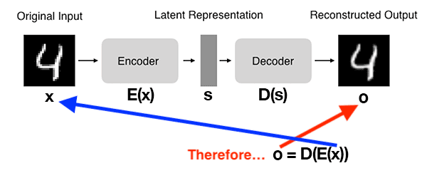
1. Encoder: Accepts the input data and compresses it into the latent-space. If we denote our input data as and the encoder as , then the output latent-space representation, , would be .
2. Decoder: The decoder is responsible for accepting the latent-space representation and then reconstructing the original input. If we denote the decoder function as and the output of the detector as , then we can represent the decoder as .

Using our mathematical notation, the entire training process of the autoencoder can be written as:

Figure 1 below demonstrates the basic architecture of an autoencoder:

Here you can see that:

1. We input a digit to the autoencoder.
2. The encoder subnetwork creates a latent representation of the digit. This latent representation is substantially smaller (in terms of dimensionality) than the input.
3. The decoder subnetwork then reconstructs the original digit from the latent representation.

You can thus think of an autoencoder as a network that reconstructs its input!

To train an autoencoder, we input our data, attempt to reconstruct it, and then minimize the mean squared error (or similar loss function).

Ideally, the output of the autoencoder will be near identical to the input.

An autoencoder reconstructs it’s input — so what’s the big deal?

At this point, some of you might be thinking:

Adrian, what’s the big deal here?

If the goal of an autoencoder is just to reconstruct the input, why even use the network in the first place?

If I wanted a copy of my input data, I could literally just copy it with a single function call.

Why on earth would I apply deep learning and go through the trouble of training a network?

This question, although a legitimate one, does indeed contain a large misconception regarding autoencoders.

Yes, during the training process, our goal is to train a network that can learn how to reconstruct our input data — but the true value of the autoencoder lives inside that latent-space representation.

Keep in mind that autoencoders compress our input data and, more to the point, when we train autoencoders, what we really care about is the encoder, , and the latent-space representation, .

The decoder, , is used to train the autoencoder end-to-end, but in practical applications, we often (but not always) care more about the encoder and the latent-space.

Later in this tutorial, we’ll be training an autoencoder on the MNIST dataset. The MNIST dataset consists of digits that are 28×28 pixels with a single channel, implying that each digit is represented by 28 x 28 = 784 values. The autoencoder we’ll be training here will be able to compress those digits into a vector of only 16 values — that’s a reduction of nearly 98%!

So what can we do if an input data point is compressed into such a small vector?

That’s where things get really interesting.

What are applications of autoencoders?

Autoencoders are typically used for:

• Dimensionality reduction (i.e., think PCA but more powerful/intelligent).
• Denoising (ex., removing noise and preprocessing images to improve OCR accuracy).
• Anomaly/outlier detection (ex., detecting mislabeled data points in a dataset or detecting when an input data point falls well outside our typical data distribution).

Outside of the computer vision field, you’ll see autoencoders applied to Natural Language Processing (NLP) and text comprehension problems, including understanding the semantic meaning of words, constructing word embeddings, and even text summarization.

How are autoencoders different from GANs?

If you’ve done any prior work with Generative Adversarial Networks (GANs), you might be wondering how autoencoders are different from GANs.

Both GANs and autoencoders are generative models; however, an autoencoder is essentially learning an identity function via compression.

The autoencoder will accept our input data, compress it down to the latent-space representation, and then attempt to reconstruct the input using just the latent-space vector.

Typically, the latent-space representation will have much fewer dimensions than the original input data.

GANs on the other hand:

1. Accept a low dimensional input.
2. Build a high dimensional space from it.
3. Generate the final output, which is not part of the original training data but ideally passes as such.

Furthermore, GANs have an evolving loss landscape, which autoencoders do not.

As a GAN is trained, the generative model generates “fake” images that are then mixed with actual “real” images — the discriminator model must then determine which images are “real” vs. “fake/generated”.

As the generative model becomes better and better at generating fake images that can fool the discriminator, the loss landscape evolves and changes (this is one of the reasons why training GANs is so damn hard).

While both GANs and autoencoders are generative models, most of their similarities end there.

Autoencoders cannot generate new, realistic data points that could be considered “passable” by humans. Instead, autoencoders are primarily used as a method to compress input data points into a latent-space representation. That latent-space representation can then be used for compression, denoising, anomaly detection, etc.

For more details on the differences between GANs and autoencoders, I suggest giving this thread on Quora a read.

Configuring your development environment

To follow along with today’s tutorial on autoencoders, you should use TensorFlow 2.0. I have two installation tutorials for TF 2.0 and associated packages to bring your development system up to speed:

• How to install TensorFlow 2.0 on Ubuntu (Ubuntu 18.04 OS; CPU and optional NVIDIA GPU)
• How to install TensorFlow 2.0 on macOS (Catalina and Mojave OSes)

Please note: PyImageSearch does not support Windows — refer to our FAQ.

Project structure

Be sure to grab the “Downloads” associated with the blog post. From there, extract the .zip and inspect the file/folder layout:

$ tree --dirsfirst
.
├── pyimagesearch
│   ├── __init__.py
│   └── convautoencoder.py
├── output.png
├── plot.png
└── train_conv_autoencoder.py

1 directory, 5 files

We will review two Python scripts today:

• convautoencoder.py: Contains the ConvAutoencoder class and build method required to assemble our neural network with tf.keras.
• train_conv_autoencoder.py: Trains a digits autoencoder on the MNIST dataset. Once the autoencoder is trained, we’ll loop over a number of output examples and write them to disk for later inspection.

Our training script results in both a plot.png figure and output.png image. The output image contains side-by-side samples of the original versus reconstructed image.

In the next section, we will implement our autoencoder with the high-level Keras API built into TensorFlow.

Implementing a convolutional autoencoder with Keras and TensorFlow

Before we can train an autoencoder, we first need to implement the autoencoder architecture itself.

To do so, we’ll be using Keras and TensorFlow.

My implementation loosely follows Francois Chollet’s own implementation of autoencoders on the official Keras blog. My primary contribution here is to go into a bit more detail regarding the implementation itself.

Open up the convautoencoder.py file in your project structure, and insert the following code:

# import the necessary packages
from tensorflow.keras.layers import BatchNormalization
from tensorflow.keras.layers import Conv2D
from tensorflow.keras.layers import Conv2DTranspose
from tensorflow.keras.layers import LeakyReLU
from tensorflow.keras.layers import Activation
from tensorflow.keras.layers import Flatten
from tensorflow.keras.layers import Dense
from tensorflow.keras.layers import Reshape
from tensorflow.keras.layers import Input
from tensorflow.keras.models import Model
from tensorflow.keras import backend as K
import numpy as np

class ConvAutoencoder:
	@staticmethod
	def build(width, height, depth, filters=(32, 64), latentDim=16):
		# initialize the input shape to be "channels last" along with
		# the channels dimension itself
		# channels dimension itself
		inputShape = (height, width, depth)
		chanDim = -1

We begin with a selection of imports from tf.keras and one from NumPy. If you don’t have TensorFlow 2.0 installed on your system, refer to the “Configuring your development environment” section above.

Our ConvAutoencoder class contains one static method, build, which accepts five parameters:

• width: Width of the input image in pixels.
• height: Height of the input image in pixels.
• depth: Number of channels (i.e., depth) of the input volume.
• filters: A tuple that contains the set of filters for convolution operations. By default, this parameter includes both 32 and 64 filters.
• latentDim: The number of neurons in our fully-connected (Dense) latent vector. By default, if this parameter is not passed, the value is set to 16.

From there, we initialize the inputShape and channel dimension (we assume “channels last” ordering).

We’re now ready to initialize our input and begin adding layers to our network:

		# define the input to the encoder
		inputs = Input(shape=inputShape)
		x = inputs

		# loop over the number of filters
		for f in filters:
			# apply a CONV => RELU => BN operation
			x = Conv2D(f, (3, 3), strides=2, padding="same")(x)
			x = LeakyReLU(alpha=0.2)(x)
			x = BatchNormalization(axis=chanDim)(x)

		# flatten the network and then construct our latent vector
		volumeSize = K.int_shape(x)
		x = Flatten()(x)
		latent = Dense(latentDim)(x)

		# build the encoder model
		encoder = Model(inputs, latent, name="encoder")

Lines 25 and 26 define the input to the encoder.

With our inputs ready, we go loop over the number of filters and add our sets of CONV=>LeakyReLU=>BN layers (Lines 29-33).

Next, we flatten the network and construct our latent vector (Lines 36-38) — this is our actual latent-space representation (i.e., the “compressed” data representation).

We then build our encoder model (Line 41).

If we were to do a print(encoder.summary()) of the encoder, assuming 28×28 single channel images (depth=1) and filters=(32, 64) and latentDim=16, we would have the following:

Model: "encoder"
_________________________________________________________________
Layer (type)                 Output Shape              Param #
=================================================================
input_1 (InputLayer)         [(None, 28, 28, 1)]       0
_________________________________________________________________
conv2d (Conv2D)              (None, 14, 14, 32)        320
_________________________________________________________________
leaky_re_lu (LeakyReLU)      (None, 14, 14, 32)        0
_________________________________________________________________
batch_normalization (BatchNo (None, 14, 14, 32)        128
_________________________________________________________________
conv2d_1 (Conv2D)            (None, 7, 7, 64)          18496
_________________________________________________________________
leaky_re_lu_1 (LeakyReLU)    (None, 7, 7, 64)          0
_________________________________________________________________
batch_normalization_1 (Batch (None, 7, 7, 64)          256
_________________________________________________________________
flatten (Flatten)            (None, 3136)              0
_________________________________________________________________
dense (Dense)                (None, 16)                50192
=================================================================
Total params: 69,392
Trainable params: 69,200
Non-trainable params: 192
_________________________________________________________________

Here we can observe that:

• Our encoder begins by accepting a 28x28x1 input volume.
• We then apply two rounds of CONV=>RELU=>BN, each with 3×3 strided convolution. The strided convolution allows us to reduce the spatial dimensions of our volumes.
• After applying our final batch normalization, we end up with a 7x7x64 volume, which is flattened into a 3136-dim vector.
• Our fully-connected layer (i.e., the Dense layer) serves our as our latent-space representation.

Next, let’s learn how the decoder model can take this latent-space representation and reconstruct the original input image:

		# start building the decoder model which will accept the
		# output of the encoder as its inputs
		latentInputs = Input(shape=(latentDim,))
		x = Dense(np.prod(volumeSize[1:]))(latentInputs)
		x = Reshape((volumeSize[1], volumeSize[2], volumeSize[3]))(x)

		# loop over our number of filters again, but this time in
		# reverse order
		for f in filters[::-1]:
			# apply a CONV_TRANSPOSE => RELU => BN operation
			x = Conv2DTranspose(f, (3, 3), strides=2,
				padding="same")(x)
			x = LeakyReLU(alpha=0.2)(x)
			x = BatchNormalization(axis=chanDim)(x)

To start building the decoder model, we:

• Construct the input to the decoder model based on the latentDim. (Lines 45 and 46).
• Accept the 1D latentDim vector and turn it into a 2D volume so that we can start applying convolution (Line 47).
• Loop over the number of filters, this time in reverse order while applying a CONV_TRANSPOSE => RELU => BN operation (Lines 51-56).

Transposed convolution is used to increase the spatial dimensions (i.e., width and height) of the volume.

Let’s finish creating our autoencoder:

		# apply a single CONV_TRANSPOSE layer used to recover the
		# original depth of the image
		x = Conv2DTranspose(depth, (3, 3), padding="same")(x)
		outputs = Activation("sigmoid")(x)

		# build the decoder model
		decoder = Model(latentInputs, outputs, name="decoder")

		# our autoencoder is the encoder + decoder
		autoencoder = Model(inputs, decoder(encoder(inputs)),
			name="autoencoder")

		# return a 3-tuple of the encoder, decoder, and autoencoder
		return (encoder, decoder, autoencoder)

Wrapping up, we:

• Apply a final CONV_TRANSPOSE layer used to recover the original channel depth of the image (1 channel for single channel/grayscale images or 3 channels for RGB images) on Line 60.
• Apply a sigmoid activation function (Line 61).
• Build the decoder model, and add it with the encoder to the autoencoder (Lines 64-68). The autoencoder becomes the encoder + decoder.
• Return a 3-tuple of the encoder, decoder, and autoencoder.

If we were to complete a print(decoder.summary()) operation here, we would have the following:

Model: "decoder"
_________________________________________________________________
Layer (type)                 Output Shape              Param #
=================================================================
input_2 (InputLayer)         [(None, 16)]              0
_________________________________________________________________
dense_1 (Dense)              (None, 3136)              53312
_________________________________________________________________
reshape (Reshape)            (None, 7, 7, 64)          0
_________________________________________________________________
conv2d_transpose (Conv2DTran (None, 14, 14, 64)        36928
_________________________________________________________________
leaky_re_lu_2 (LeakyReLU)    (None, 14, 14, 64)        0
_________________________________________________________________
batch_normalization_2 (Batch (None, 14, 14, 64)        256
_________________________________________________________________
conv2d_transpose_1 (Conv2DTr (None, 28, 28, 32)        18464
_________________________________________________________________
leaky_re_lu_3 (LeakyReLU)    (None, 28, 28, 32)        0
_________________________________________________________________
batch_normalization_3 (Batch (None, 28, 28, 32)        128
_________________________________________________________________
conv2d_transpose_2 (Conv2DTr (None, 28, 28, 1)         289
_________________________________________________________________
activation (Activation)      (None, 28, 28, 1)         0
=================================================================
Total params: 109,377
Trainable params: 109,185
Non-trainable params: 192
_________________________________________________________________

The decoder accepts our 16-dim latent representation from the encoder and then builds a new fully-connected layer of 3136-dim, which is the product of 7 x 7 x 64 = 3136.

Using our new 3136-dim FC layer, we reshape it into a 3D volume of 7 x 7 x 64. From there we can start applying our CONV_TRANSPOSE=>RELU=>BN operation. Unlike standard strided convolution, which is used to decrease volume size, our transposed convolution is used to increase volume size.

Finally, a transposed convolution layer is applied to recover the original channel depth of the image. Since our images are grayscale, we learn a single filter, the output of which is a 28 x 28 x 1 volume (i.e., the dimensions of the original MNIST digit images).

A print(autoencoder.summary()) operation shows the composed nature of the encoder and decoder:

Model: "autoencoder"
_________________________________________________________________
Layer (type)                 Output Shape              Param #
=================================================================
input_1 (InputLayer)         [(None, 28, 28, 1)]       0
_________________________________________________________________
encoder (Model)              (None, 16)                69392
_________________________________________________________________
decoder (Model)              (None, 28, 28, 1)         109377
=================================================================
Total params: 178,769
Trainable params: 178,385
Non-trainable params: 384
_________________________________________________________________

The input to our encoder is the original 28 x 28 x 1 images from the MNIST dataset. Our encoder then learns a 16-dim latent-space representation of the data, after which the decoder reconstructs the original 28 x 28 x 1 images.

In the next section, we will develop our script to train our autoencoder.

Creating the convolutional autoencoder training script

With our autoencoder architecture implemented, let’s move on to the training script.

Open up the train_conv_autoencoder.py in your project directory structure, and insert the following code:

# set the matplotlib backend so figures can be saved in the background
import matplotlib
matplotlib.use("Agg")

# import the necessary packages
from pyimagesearch.convautoencoder import ConvAutoencoder
from tensorflow.keras.optimizers import Adam
from tensorflow.keras.datasets import mnist
import matplotlib.pyplot as plt
import numpy as np
import argparse
import cv2

# construct the argument parse and parse the arguments
ap = argparse.ArgumentParser()
ap.add_argument("-s", "--samples", type=int, default=8,
	help="# number of samples to visualize when decoding")
ap.add_argument("-o", "--output", type=str, default="output.png",
	help="path to output visualization file")
ap.add_argument("-p", "--plot", type=str, default="plot.png",
	help="path to output plot file")
args = vars(ap.parse_args())

On Lines 2-12, we handle our imports. We’ll use the "Agg" backend of matplotlib so that we can export our training plot to disk.

We need our custom ConvAutoencoder architecture class which we implemented in the previous section.

We will use the Adam optimizer as we train on the MNIST benchmarking dataset. For visualization, we’ll employ OpenCV.

Next, we’ll parse three command line arguments, all of which are optional:

• --samples: The number of output samples for visualization. By default this value is set to 8.
• --output: The path the output visualization image. We’ll name our visualization output.png by default
• --plot: The path to our matplotlib output plot. A default of plot.png is assigned if this argument is not provided in the terminal.

Now we’ll set a couple hyperparameters and preprocess our MNIST dataset:

# initialize the number of epochs to train for and batch size
EPOCHS = 25
BS = 32

# load the MNIST dataset
print("[INFO] loading MNIST dataset...")
((trainX, _), (testX, _)) = mnist.load_data()

# add a channel dimension to every image in the dataset, then scale
# the pixel intensities to the range [0, 1]
trainX = np.expand_dims(trainX, axis=-1)
testX = np.expand_dims(testX, axis=-1)
trainX = trainX.astype("float32") / 255.0
testX = testX.astype("float32") / 255.0

Lines 25 and 26 initialize the batch size and number of training epochs.

From there, we’ll work with our MNIST dataset. TensorFlow/Keras has a handy load_data method that we can call on mnist to grab the data (Line 30). From there, Lines 34-37 (1) add a channel dimension to every image in the dataset and (2) scale the pixel intensities to the range [0, 1].

We’re now ready to build and train our autoencoder:

# construct our convolutional autoencoder
print("[INFO] building autoencoder...")
(encoder, decoder, autoencoder) = ConvAutoencoder.build(28, 28, 1)
opt = Adam(lr=1e-3)
autoencoder.compile(loss="mse", optimizer=opt)

# train the convolutional autoencoder
H = autoencoder.fit(
	trainX, trainX,
	validation_data=(testX, testX),
	epochs=EPOCHS,
	batch_size=BS)

To build the convolutional autoencoder, we call the build method on our ConvAutoencoder class and pass the necessary arguments (Line 41). Recall that this results in the (encoder, decoder, autoencoder) tuple — going forward in this script, we only need the autoencoder for training and predictions.

We initialize our Adam optimizer with an initial learning rate of 1e-3 and go ahead and compile it with mean-squared error loss (Lines 42 and 43).

From there, we fit (train) our autoencoder on the MNIST data (Lines 46-50).

Let’s go ahead and plot our training history:

# construct a plot that plots and saves the training history
N = np.arange(0, EPOCHS)
plt.style.use("ggplot")
plt.figure()
plt.plot(N, H.history["loss"], label="train_loss")
plt.plot(N, H.history["val_loss"], label="val_loss")
plt.title("Training Loss and Accuracy")
plt.xlabel("Epoch #")
plt.ylabel("Loss/Accuracy")
plt.legend(loc="lower left")
plt.savefig(args["plot"])

And from there, we’ll make predictions on our testing set:

# use the convolutional autoencoder to make predictions on the
# testing images, then initialize our list of output images
print("[INFO] making predictions...")
decoded = autoencoder.predict(testX)
outputs = None

# loop over our number of output samples
for i in range(0, args["samples"]):
	# grab the original image and reconstructed image
	original = (testX[i] * 255).astype("uint8")
	recon = (decoded[i] * 255).astype("uint8")

	# stack the original and reconstructed image side-by-side
	output = np.hstack([original, recon])

	# if the outputs array is empty, initialize it as the current
	# side-by-side image display
	if outputs is None:
		outputs = output

	# otherwise, vertically stack the outputs
	else:
		outputs = np.vstack([outputs, output])

# save the outputs image to disk
cv2.imwrite(args["output"], outputs)

Line 67 makes predictions on the test set. We then loop over the number of --samples passed as a command line argument (Line 71) so that we can build our visualization. Inside the loop, we:

• Grab both the original and reconstructed images (Lines 73 and 74).
• Stack the pair of images side-by-side (Line 77).
• Stack the pairs vertically (Lines 81-86).
• Finally, we output the visualization image to disk (Line 89).

In the next section, we’ll see the results of our hard work.

Training the convolutional autoencoder with Keras and TensorFlow

We are now ready to see our autoencoder in action!

Make sure you use the “Downloads” section of this post to download the source code — from there you can execute the following command:

$ python train_conv_autoencoder.py
[INFO] loading MNIST dataset...
[INFO] building autoencoder...
Train on 60000 samples, validate on 10000 samples
Epoch 1/25
60000/60000 [==============================] - 68s 1ms/sample - loss: 0.0188 - val_loss: 0.0108
Epoch 2/25
60000/60000 [==============================] - 68s 1ms/sample - loss: 0.0104 - val_loss: 0.0096
Epoch 3/25
60000/60000 [==============================] - 68s 1ms/sample - loss: 0.0094 - val_loss: 0.0086
Epoch 4/25
60000/60000 [==============================] - 68s 1ms/sample - loss: 0.0088 - val_loss: 0.0086
Epoch 5/25
60000/60000 [==============================] - 68s 1ms/sample - loss: 0.0084 - val_loss: 0.0080
...
Epoch 20/25
60000/60000 [==============================] - 83s 1ms/sample - loss: 0.0067 - val_loss: 0.0069
Epoch 21/25
60000/60000 [==============================] - 83s 1ms/sample - loss: 0.0066 - val_loss: 0.0069
Epoch 22/25
60000/60000 [==============================] - 83s 1ms/sample - loss: 0.0066 - val_loss: 0.0068
Epoch 23/25
60000/60000 [==============================] - 83s 1ms/sample - loss: 0.0066 - val_loss: 0.0068
Epoch 24/25
60000/60000 [==============================] - 83s 1ms/sample - loss: 0.0065 - val_loss: 0.0067
Epoch 25/25
60000/60000 [==============================] - 83s 1ms/sample - loss: 0.0065 - val_loss: 0.0068
[INFO] making predictions...

As Figure 4 and the terminal output demonstrate, our training process was able to minimize the reconstruction loss of the autoencoder.

But how well did the autoencoder do at reconstructing the training data?

The answer is very good:

In Figure 5, on the left is our original image while the right is the reconstructed digit predicted by the autoencoder. As you can see, the digits are nearly indistinguishable from each other!

At this point, you may be thinking:

Great … so I can train a network to reconstruct my original image.

But you said that what really matters is the internal latent-space representation.

How can I access that representation, and how can I use it for denoising and anomaly/outlier detection?

Those are great questions — I’ll be addressing both in my next two tutorials here on PyImageSearch, so stay tuned!

What’s next?

This tutorial and the next two in this series admittedly discuss advanced applications of computer vision and deep learning.

If you don’t already know the fundamentals of deep learning, now would be a good time to learn them. To get a head start, I personally suggest you read my book, Deep Learning for Computer Vision with Python.

Inside the book, you will learn:

• Deep learning fundamentals and theory without unnecessary mathematical fluff. I present the basic equations and back them up with code walkthroughs that you can implement and easily understand. You don’t need a degree in advanced mathematics to understand this book.
• How to implement your own custom neural network architectures. Not only will you learn how to implement state-of-the-art architectures, including ResNet, SqueezeNet, etc., but you’ll also learn how to create your own custom CNNs.
• How to train CNNs on your own datasets. Most deep learning tutorials don’t teach you how to work with your own custom datasets. Mine do. You’ll be training CNNs on your own datasets in no time.
• Object detection (Faster R-CNNs, Single Shot Detectors, and RetinaNet) and instance segmentation (Mask R-CNN). Use these chapters to create your own custom object detectors and segmentation networks.

If you’re interested in learning more about the book, I’d be happy to send you a free PDF containing the Table of Contents and a few sample chapters. Simply click the button below:

Summary

In this tutorial, you learned the fundamentals of autoencoders.

Autoencoders are generative models that consist of an encoder and a decoder model. When trained, the encoder takes input data point and learns a latent-space representation of the data. This latent-space representation is a compressed representation of the data, allowing the model to represent it in far fewer parameters than the original data.

The decoder model then takes the latent-space representation and attempts to reconstruct the original data point from it. When trained end-to-end, the encoder and decoder function in a composed manner.

In practice, we use autoencoders for dimensionality reduction, compression, denoising, and anomaly detection.

After we understood the fundamentals, we implemented a convolutional autoencoder using Keras and TensorFlow.

In next week’s tutorial, we’ll learn how to use a convolutional autoencoder for denoising.

To download the source code to this post (and be notified when future tutorials are published here on PyImageSearch), just enter your email address in the form below!

Download the Source Code and FREE 17-page Resource Guide

Enter your email address below to get a .zip of the code and a FREE 17-page Resource Guide on Computer Vision, OpenCV, and Deep Learning. Inside you’ll find my hand-picked tutorials, books, courses, and libraries to help you master CV and DL!

Download the code!

Website

The post Autoencoders with Keras, TensorFlow, and Deep Learning appeared first on PyImageSearch.

In this tutorial, you will learn how to use autoencoders to denoise images using Keras, TensorFlow, and Deep Learning.

Today’s tutorial is part two in our three-part series on the applications of autoencoders:

1. Autoencoders with Keras, TensorFlow, and Deep Learning (last week’s tutorial)
2. Denoising autoenecoders with Keras, TensorFlow and Deep Learning (today’s tutorial)
3. Anomaly detection with Keras, TensorFlow, and Deep Learning (next week’s tutorial)

Last week you learned the fundamentals of autoencoders, including how to train your very first autoencoder using Keras and TensorFlow — however, the real-world application of that tutorial was admittedly a bit limited due to the fact that we needed to lay the groundwork.

Today, we’re going to take a deeper dive and learn how autoencoders can be used for denoising, also called “noise reduction,” which is the process of removing noise from a signal.

The term “noise” here could be:

• Produced by a faulty or poor quality image sensor
• Random variations in brightness or color
• Quantization noise
• Artifacts due to JPEG compression
• Image perturbations produced by an image scanner or threshold post-processing
• Poor paper quality (crinkles and folds) when trying to perform OCR

From the perspective of image processing and computer vision, you should think of noise as anything that could be removed by a really good pre-processing filter.

Our goal is to train an autoencoder to perform such pre-processing — we call such models denoising autoencoders.

To learn how to train a denoising autoencoder with Keras and TensorFlow, just keep reading!

Looking for the source code to this post?

Jump Right To The Downloads Section

Denoising autoencoders with Keras, TensorFlow, and Deep Learning

In the first part of this tutorial, we’ll discuss what denoising autoencoders are and why we may want to use them.

From there I’ll show you how to implement and train a denoising autoencoder using Keras and TensorFlow.

We’ll wrap up this tutorial by examining the results of our denoising autoencoder.

What are denoising autoencoders, and why would we use them?

Denoising autoencoders are an extension of simple autoencoders; however, it’s worth noting that denoising autoencoders were not originally meant to automatically denoise an image.

Instead, the denoising autoencoder procedure was invented to help:

• The hidden layers of the autoencoder learn more robust filters
• Reduce the risk of overfitting in the autoencoder
• Prevent the autoencoder from learning a simple identify function

In Vincent et al.’s 2008 ICML paper, Extracting and Composing Robust Features with Denoising Autoencoders, the authors found that they could improve the robustness of their internal layers (i.e., latent-space representation) by purposely introducing noise to their signal.

Noise was stochastically (i.e., randomly) added to the input data, and then the autoencoder was trained to recover the original, nonperturbed signal.

From an image processing standpoint, we can train an autoencoder to perform automatic image pre-processing for us.

A great example would be pre-processing an image to improve the accuracy of an optical character recognition (OCR) algorithm. If you’ve ever applied OCR before, you know how just a little bit of the wrong type of noise (ex., printer ink smudges, poor image quality during the scan, etc.) can dramatically hurt the performance of your OCR method. Using denoising autoencoders, we can automatically pre-process the image, improve the quality, and therefore increase the accuracy of the downstream OCR algorithm.

If you’re interested in learning more about denoising autoencoders, I would strongly encourage you to read this article as well Bengio and Delalleau’s paper, Justifying and Generalizing Contrastive Divergence.

For more information on denoising autoencoders for OCR-related preprocessing, take a look at this dataset on Kaggle.

Configuring your development environment

To follow along with today’s tutorial on autoencoders, you should use TensorFlow 2.0. I have two installation tutorials for TF 2.0 and associated packages to bring your development system up to speed:

• How to install TensorFlow 2.0 on Ubuntu (Ubuntu 18.04 OS; CPU and optional NVIDIA GPU)
• How to install TensorFlow 2.0 on macOS (Catalina and Mojave OSes)

Please note: PyImageSearch does not support Windows — refer to our FAQ.

Project structure

Go ahead and grab the .zip from the “Downloads” section of today’s tutorial. From there, extract the zip.

You’ll be presented with the following project layout:

$ tree --dirsfirst
.
├── pyimagesearch
│   ├── __init__.py
│   └── convautoencoder.py
├── output.png
├── plot.png
└── train_denoising_autoencoder.py

1 directory, 5 files

The pyimagesearch module contains the ConvAutoencoder class. We reviewed this class in our previous tutorial; however, we’ll briefly walk through it again today.

The heart of today’s tutorial is inside the train_denoising_autoencoder.py Python training script. This script is different from the previous tutorial in one main way:

We will purposely add noise to our MNIST training images using a random normal distribution centered at 0.5 with a standard deviation of 0.5.

The purpose of adding noise to our training data is so that our autoencoder can effectively remove noise from an input image (i.e., denoise).

Implementing our denoising autoencoder with Keras and TensorFlow

The denoising autoencoder we’ll be implementing today is essentially identical to the one we implemented in last week’s tutorial on autoencoder fundamentals.

We’ll review the model architecture here today as a matter of completeness, but make sure you refer to last week’s guide for more details.

With that said, open up the convautoencoder.py file in your project structure, and insert the following code:

# import the necessary packages
from tensorflow.keras.layers import BatchNormalization
from tensorflow.keras.layers import Conv2D
from tensorflow.keras.layers import Conv2DTranspose
from tensorflow.keras.layers import LeakyReLU
from tensorflow.keras.layers import Activation
from tensorflow.keras.layers import Flatten
from tensorflow.keras.layers import Dense
from tensorflow.keras.layers import Reshape
from tensorflow.keras.layers import Input
from tensorflow.keras.models import Model
from tensorflow.keras import backend as K
import numpy as np

class ConvAutoencoder:
	@staticmethod
	def build(width, height, depth, filters=(32, 64), latentDim=16):
		# initialize the input shape to be "channels last" along with
		# the channels dimension itself
		# channels dimension itself
		inputShape = (height, width, depth)
		chanDim = -1

		# define the input to the encoder
		inputs = Input(shape=inputShape)
		x = inputs

Imports include tf.keras and NumPy.

Our ConvAutoencoder class contains one static method, build which accepts five parameters:

• width: Width of the input image in pixels
• height: Heigh of the input image in pixels
• depth: Number of channels (i.e., depth) of the input volume
• filters: A tuple that contains the set of filters for convolution operations. By default, if this parameter is not provided by the caller, we’ll add two sets of CONV => RELU => BN with 32 and 64 filters
• latentDim: The number of neurons in our fully-connected (Dense) latent vector. By default, if this parameter is not passed, the value is set to 16

From there, we initialize the inputShape and define the Input to the encoder (Lines 25 and 26).

Let’s begin building our encoder’s filters:

		# loop over the number of filters
		for f in filters:
			# apply a CONV => RELU => BN operation
			x = Conv2D(f, (3, 3), strides=2, padding="same")(x)
			x = LeakyReLU(alpha=0.2)(x)
			x = BatchNormalization(axis=chanDim)(x)

		# flatten the network and then construct our latent vector
		volumeSize = K.int_shape(x)
		x = Flatten()(x)
		latent = Dense(latentDim)(x)

		# build the encoder model
		encoder = Model(inputs, latent, name="encoder")

Using Keras’ functional API, we go ahead and Loop over number of filters and add our sets of CONV => RELU => BN layers (Lines 29-33).

We then flatten the network and construct our latent vector (Lines 36-38). The latent-space representation is the compressed form of our data.

From there, we build the encoder portion of our autoencoder (Line 41).

Next, we’ll use our latent-space representation to reconstruct the original input image.

		# start building the decoder model which will accept the
		# output of the encoder as its inputs
		latentInputs = Input(shape=(latentDim,))
		x = Dense(np.prod(volumeSize[1:]))(latentInputs)
		x = Reshape((volumeSize[1], volumeSize[2], volumeSize[3]))(x)

		# loop over our number of filters again, but this time in
		# reverse order
		for f in filters[::-1]:
			# apply a CONV_TRANSPOSE => RELU => BN operation
			x = Conv2DTranspose(f, (3, 3), strides=2,
				padding="same")(x)
			x = LeakyReLU(alpha=0.2)(x)
			x = BatchNormalization(axis=chanDim)(x)

		# apply a single CONV_TRANSPOSE layer used to recover the
		# original depth of the image
		x = Conv2DTranspose(depth, (3, 3), padding="same")(x)
		outputs = Activation("sigmoid")(x)

		# build the decoder model
		decoder = Model(latentInputs, outputs, name="decoder")

		# our autoencoder is the encoder + decoder
		autoencoder = Model(inputs, decoder(encoder(inputs)),
			name="autoencoder")

		# return a 3-tuple of the encoder, decoder, and autoencoder
		return (encoder, decoder, autoencoder)

Here, we are taking the latent input and use a fully-connected layer to reshape it into a 3D volume (i.e., the image data).

We loop over our filters again, but in reverse order, applying CONV_TRANSPOSE => RELU => BN layers where the CONV_TRANSPOSE layer’s purpose is to increase the volume size.

Finally, we build the decoder model and construct the autoencoder. Remember, the concept of an autoencoder — discussed last week — consists of both the encoder and decoder components.

Implementing the denoising autoencoder training script

Let’s now implement the training script used to:

1. Add stochastic noise to the MNIST dataset
2. Train a denoising autoencoder on the noisy dataset
3. Automatically recover the original digits from the noise

My implementation follows Francois Chollet’s own implementation of denoising autoencoders on the official Keras blog — my primary contribution here is to go into a bit more detail regarding the implementation itself.

Open up the train_denoising_autoencoder.py file, and insert the following code:

# set the matplotlib backend so figures can be saved in the background
import matplotlib
matplotlib.use("Agg")

# import the necessary packages
from pyimagesearch.convautoencoder import ConvAutoencoder
from tensorflow.keras.optimizers import Adam
from tensorflow.keras.datasets import mnist
import matplotlib.pyplot as plt
import numpy as np
import argparse
import cv2

# construct the argument parse and parse the arguments
ap = argparse.ArgumentParser()
ap.add_argument("-s", "--samples", type=int, default=8,
	help="# number of samples to visualize when decoding")
ap.add_argument("-o", "--output", type=str, default="output.png",
	help="path to output visualization file")
ap.add_argument("-p", "--plot", type=str, default="plot.png",
	help="path to output plot file")
args = vars(ap.parse_args())

On Lines 2-12 we handle our imports. We’ll use the "Agg" backend of matplotlib so that we can export our training plot to disk. Our custom ConvAutoencoder class implemented in the previous section contains the autoencoder architecture itself. Modeling after Chollet’s example, we will also use the Adam optimizer.

Our script accepts three optional command line arguments:

• --samples: The number of output samples for visualization. By default this value is set to 8.
• --output: The path to the output visualization image. We’ll name our visualization output.png by default.
• --plot: The path to our matplotlib output plot. A default of plot.png is assigned if this argument is not provided in the terminal.

Next, we initialize hyperparameters and preprocess our MNIST dataset:

# initialize the number of epochs to train for and batch size
EPOCHS = 25
BS = 32

# load the MNIST dataset
print("[INFO] loading MNIST dataset...")
((trainX, _), (testX, _)) = mnist.load_data()

# add a channel dimension to every image in the dataset, then scale
# the pixel intensities to the range [0, 1]
trainX = np.expand_dims(trainX, axis=-1)
testX = np.expand_dims(testX, axis=-1)
trainX = trainX.astype("float32") / 255.0
testX = testX.astype("float32") / 255.0

Our training epochs will be 25 and we’ll use a batch size of 32.

We go ahead and grab the MNIST dataset (Line 30) while Lines 34-37 (1) add a channel dimension to every image in the dataset, and (2) scale the pixel intensities to the range [0, 1].

At this point, we’ll deviate from last week’s tutorial:

# sample noise from a random normal distribution centered at 0.5 (since
# our images lie in the range [0, 1]) and a standard deviation of 0.5
trainNoise = np.random.normal(loc=0.5, scale=0.5, size=trainX.shape)
testNoise = np.random.normal(loc=0.5, scale=0.5, size=testX.shape)
trainXNoisy = np.clip(trainX + trainNoise, 0, 1)
testXNoisy = np.clip(testX + testNoise, 0, 1)

To add random noise to the MNIST digits, we use NumPy’s random normal distribution centered at 0.5 with a standard deviation of 0.5 (Lines 41-44).

The following figure shows an example of how our images look before (left) adding noise followed by after (right):

As you can see, our images are quite corrupted — recovering the original digit from the noise will require a powerful model.

Luckily, our denoising autoencoder will be up to the task:

# construct our convolutional autoencoder
print("[INFO] building autoencoder...")
(encoder, decoder, autoencoder) = ConvAutoencoder.build(28, 28, 1)
opt = Adam(lr=1e-3)
autoencoder.compile(loss="mse", optimizer=opt)

# train the convolutional autoencoder
H = autoencoder.fit(
	trainXNoisy, trainX,
	validation_data=(testXNoisy, testX),
	epochs=EPOCHS,
	batch_size=BS)

# construct a plot that plots and saves the training history
N = np.arange(0, EPOCHS)
plt.style.use("ggplot")
plt.figure()
plt.plot(N, H.history["loss"], label="train_loss")
plt.plot(N, H.history["val_loss"], label="val_loss")
plt.title("Training Loss and Accuracy")
plt.xlabel("Epoch #")
plt.ylabel("Loss/Accuracy")
plt.legend(loc="lower left")
plt.savefig(args["plot"])

Line 48 builds our denoising autoencoder, passing the necessary arguments. Using our Adam optimizer with an initial learning rate of 1e-3, we go ahead and compile the autoencoder with mean-squared error loss (Lines 49 and 50).

Training is launched via Lines 53-57. Using the training history data, H, Lines 60-69 plot the loss, saving the resulting figure to disk.

Let’s write a quick loop that will help us visualize the denoising autoencoder results:

# use the convolutional autoencoder to make predictions on the
# testing images, then initialize our list of output images
print("[INFO] making predictions...")
decoded = autoencoder.predict(testX)
outputs = None

# loop over our number of output samples
for i in range(0, args["samples"]):
	# grab the original image and reconstructed image
	original = (testXNoisy[i] * 255).astype("uint8")
	recon = (decoded[i] * 255).astype("uint8")

	# stack the original and reconstructed image side-by-side
	output = np.hstack([original, recon])

	# if the outputs array is empty, initialize it as the current
	# side-by-side image display
	if outputs is None:
		outputs = output

	# otherwise, vertically stack the outputs
	else:
		outputs = np.vstack([outputs, output])

# save the outputs image to disk
cv2.imwrite(args["output"], outputs)

We go ahead and use our trained autoencoder to remove the noise from the images in our testing set (Line 74).

We then grab N --samples worth of original and reconstructed data, and put together a visualization montage (Lines 78-93). Line 96 writes the visualization figure to disk for inspection.

Training the denoising autoencoder with Keras and TensorFlow

To train your denoising autoencoder, make sure you use the “Downloads” section of this tutorial to download the source code.

From there, open up a terminal and execute the following command:

$ python train_denoising_autoencoder.py --output output_denoising.png \
	--plot plot_denoising.png
[INFO] loading MNIST dataset...
[INFO] building autoencoder...
Train on 60000 samples, validate on 10000 samples
Epoch 1/25
60000/60000 [==============================] - 85s 1ms/sample - loss: 0.0285 - val_loss: 0.0191
Epoch 2/25
60000/60000 [==============================] - 83s 1ms/sample - loss: 0.0187 - val_loss: 0.0211
Epoch 3/25
60000/60000 [==============================] - 84s 1ms/sample - loss: 0.0177 - val_loss: 0.0174
Epoch 4/25
60000/60000 [==============================] - 84s 1ms/sample - loss: 0.0171 - val_loss: 0.0170
Epoch 5/25
60000/60000 [==============================] - 83s 1ms/sample - loss: 0.0167 - val_loss: 0.0177
...
Epoch 21/25
60000/60000 [==============================] - 67s 1ms/sample - loss: 0.0146 - val_loss: 0.0161
Epoch 22/25
60000/60000 [==============================] - 67s 1ms/sample - loss: 0.0145 - val_loss: 0.0164
Epoch 23/25
60000/60000 [==============================] - 67s 1ms/sample - loss: 0.0145 - val_loss: 0.0158
Epoch 24/25
60000/60000 [==============================] - 67s 1ms/sample - loss: 0.0144 - val_loss: 0.0155
Epoch 25/25
60000/60000 [==============================] - 66s 1ms/sample - loss: 0.0144 - val_loss: 0.0157
[INFO] making predictions...

Training the denoising autoencoder on my iMac Pro with a 3 GHz Intel Xeon W processor took ~32.20 minutes.

As Figure 3 shows, our training process was stable and shows no signs of overfitting.

Denoising autoencoder results

Our denoising autoencoder has been successfully trained, but how did it perform when removing the noise we added to the MNIST dataset?

To answer that question, take a look at Figure 4:

On the left we have the original MNIST digits that we added noise to while on the right we have the output of the denoising autoencoder — we can clearly see that the denoising autoencoder was able to recover the original signal (i.e., digit) from the image while removing the noise.

More advanced denosing autoencoders can be used to automatically pre-process images to facilitate better OCR accuracy.

What’s next?

The path I took as I entered the field of deep learning and worked my way up to becoming an expert was not straightforward.

It was a grueling process of reading academic papers (some good, some junk), trying to figure out what all the terms mean, and trying to implement deep learning architectures from scratch. I became frustrated with my failed attempts at implementation, spending hours and days searching on Google, hunting for deep learning tutorials.

Back then, there weren’t many deep learning tutorials to be found, and while I also had some books stacked on my desk, they were too heavy with mathematical notation that professors thought would actually be useful to the average student.

Let’s face it, these days most of us don’t want to implement gradient descent or backpropagation algorithms by hand. While it can be a great learning exercise if you plan to write a dissertation on an improvement to the algorithm, we just want to learn how to train models on custom data.

In the age of internet-content-clickbait shared on social media, don’t blindly follow poorly written blog posts from nonreputable sources that you stumble upon. While free can be good, ultimately you get what you pay for.

Ask yourself:

• Do you want to hop around learning in an ad hoc manner, risking getting lost in the mess of free content available all over the net?
• Or do you want to study with the linear path that my deep learning book presents, arming you with a solid foundation with which you can build upon to study more advanced techniques?

Don’t study the way I did. It can be a great way to learn, but it isn’t efficient, and too many people find themselves giving up.

Instead, grab my book, Deep Learning for Computer Vision with Python so you can study the right way.

I crafted my book so that it perfectly balances theory with implementation, ensuring you properly master:

• Deep learning fundamentals and theory without unnecessary mathematical fluff. I present the basic equations and back them up with code walkthroughs that you can implement and easily understand. You don’t need a degree in advanced mathematics to understand this book.
• How to implement your own custom neural network architectures. Not only will you learn how to implement state-of-the-art architectures, including ResNet, SqueezeNet, etc., but you’ll also learn how to create your own custom CNNs.
• How to train CNNs on your own datasets. Most deep learning tutorials don’t teach you how to work with your own custom datasets. Mine do. You’ll be training CNNs on your own datasets in no time.
• Object detection (Faster R-CNNs, Single Shot Detectors, and RetinaNet) and instance segmentation (Mask R-CNN). Use these chapters to create your own custom object detectors and segmentation networks.

If you’re interested in learning more about the book, I’d be happy to send you a free PDF containing the Table of Contents and a few sample chapters:

Summary

In this tutorial, you learned about denoising autoencoders, which, as the name suggests, are models that are used to remove noise from a signal.

In the context of computer vision, denoising autoencoders can be seen as very powerful filters that can be used for automatic pre-processing. For example, a denoising autoencoder could be used to automatically pre-process an image, improving its quality for an OCR algorithm and thereby increasing OCR accuracy.

To demonstrate a denoising autoencoder in action, we added noise to the MNIST dataset, greatly degrading the image quality to the point where any model would struggle to correctly classify the digit in the image. Using our denoising autoencoder, we were able to remove the noise from the image, recovering the original signal (i.e., the digit).

In next week’s tutorial, you’ll learn about another real-world application of autoencoders — anomaly and outlier detection.

To download the source code to this post (and be notified when future tutorials are published here on PyImageSearch), just enter your email address in the form below!

Download the Source Code and FREE 17-page Resource Guide

Enter your email address below to get a .zip of the code and a FREE 17-page Resource Guide on Computer Vision, OpenCV, and Deep Learning. Inside you’ll find my hand-picked tutorials, books, courses, and libraries to help you master CV and DL!

Download the code!

Website

The post Denoising autoencoders with Keras, TensorFlow, and Deep Learning appeared first on PyImageSearch.

In this tutorial, you will learn how to perform anomaly and outlier detection using autoencoders, Keras, and TensorFlow.

Back in January, I showed you how to use standard machine learning models to perform anomaly detection and outlier detection in image datasets.

Our approach worked well enough, but it begged the question:

Could deep learning be used to improve the accuracy of our anomaly detector?

To answer such a question would require us to dive further down the rabbit hole and answer questions such as:

• What model architecture should we use?
• Are some deep neural network architectures better than others for anomaly/outlier detection?
• How do we handle the class imbalance problem?
• What if we wanted to train an unsupervised anomaly detector?

This tutorial addresses all of these questions, and by the end of it, you’ll be able to perform anomaly detection in your own image datasets using deep learning.

To learn how to perform anomaly detection with Keras, TensorFlow, and Deep Learning, just keep reading!

Looking for the source code to this post?

Jump Right To The Downloads Section

Anomaly detection with Keras, TensorFlow, and Deep Learning

In the first part of this tutorial, we’ll discuss anomaly detection, including:

• What makes anomaly detection so challenging
• Why traditional deep learning methods are not sufficient for anomaly/outlier detection
• How autoencoders can be used for anomaly detection

From there, we’ll implement an autoencoder architecture that can be used for anomaly detection using Keras and TensorFlow. We’ll then train our autoencoder model in an unsupervised fashion.

Once the autoencoder is trained, I’ll show you how you can use the autoencoder to identify outliers/anomalies in both your training/testing set as well as in new images that are not part of your dataset splits.

What is anomaly detection?

To quote my intro to anomaly detection tutorial:

Anomalies are defined as events that deviate from the standard, happen rarely, and don’t follow the rest of the “pattern.”

Examples of anomalies include:

• Large dips and spikes in the stock market due to world events
• Defective items in a factory/on a conveyor belt
• Contaminated samples in a lab

Depending on your exact use case and application, anomalies only typically occur 0.001-1% of the time — that’s an incredibly small fraction of the time.

The problem is only compounded by the fact that there is a massive imbalance in our class labels.

By definition, anomalies will rarely occur, so the majority of our data points will be of valid events.

To detect anomalies, machine learning researchers have created algorithms such as Isolation Forests, One-class SVMs, Elliptic Envelopes, and Local Outlier Factor to help detect such events; however, all of these methods are rooted in traditional machine learning.

What about deep learning?

Can deep learning be used for anomaly detection as well?

The answer is yes — but you need to frame the problem correctly.

How can deep learning and autoencoders be used for anomaly detection?

As I discussed in my intro to autoencoder tutorial, autoencoders are a type of unsupervised neural network that can:

1. Accept an input set of data
2. Internally compress the data into a latent-space representation
3. Reconstruct the input data from the latent representation

To accomplish this task, an autoencoder uses two components: an encoder and a decoder.

The encoder accepts the input data and compresses it into the latent-space representation. The decoder then attempts to reconstruct the input data from the latent space.

When trained in an end-to-end fashion, the hidden layers of the network learn filters that are robust and even capable of denoising the input data.

However, what makes autoencoders so special from an anomaly detection perspective is the reconstruction loss. When we train an autoencoder, we typically measure the mean-squared-error (MSE) between:

1. The input image
2. The reconstructed image from the autoencoder

The lower the loss, the better a job the autoencoder is doing at reconstructing the image.

Let’s now suppose that we trained an autoencoder on the entirety of the MNIST dataset:

We then present the autoencoder with a digit and tell it to reconstruct it:

We would expect the autoencoder to do a really good job at reconstructing the digit, as that is exactly what the autoencoder was trained to do — and if we were to look at the MSE between the input image and the reconstructed image, we would find that it’s quite low.

Let’s now suppose we presented our autoencoder with a photo of an elephant and asked it to reconstruct it:

Since the autoencoder has never seen an elephant before, and more to the point, was never trained to reconstruct an elephant, our MSE will be very high.

If the MSE of the reconstruction is high, then we likely have an outlier.

Alon Agmon does a great job explaining this concept in more detail in this article.

Configuring your development environment

To follow along with today’s tutorial on anomaly detection, I recommend you use TensorFlow 2.0.

To configure your system and install TensorFlow 2.0, you can follow either my Ubuntu or macOS guide:

• How to install TensorFlow 2.0 on Ubuntu (Ubuntu 18.04 OS; CPU and optional NVIDIA GPU)
• How to install TensorFlow 2.0 on macOS (Catalina and Mojave OSes)

Please note: PyImageSearch does not support Windows — refer to our FAQ.

Project structure

Go ahead and grab the code from the “Downloads” section of this post. Once you’ve unzipped the project, you’ll be presented with the following structure:

$ tree --dirsfirst
.
├── output
│   ├── autoencoder.model
│   └── images.pickle
├── pyimagesearch
│   ├── __init__.py
│   └── convautoencoder.py
├── find_anomalies.py
├── plot.png
├── recon_vis.png
└── train_unsupervised_autoencoder.py

2 directories, 8 files

Our convautoencoder.py file contains the ConvAutoencoder class which is responsible for building a Keras/TensorFlow autoencoder implementation.

We will train an autoencoder with unlabeled data inside train_unsupervised_autoencoder.py, resulting in the following outputs:

• autoencoder.model: The serialized, trained autoencoder model.
• images.pickle: A serialized set of unlabeled images for us to find anomalies in.
• plot.png: A plot consisting of our training loss curves.
• recon_vis.png: A visualization figure that compares samples of ground-truth digit images versus each reconstructed image.

From there, we will develop an anomaly detector inside find_anomalies.py and apply our autoencoder to reconstruct data and find anomalies.

Implementing our autoencoder for anomaly detection with Keras and TensorFlow

The first step to anomaly detection with deep learning is to implement our autoencoder script.

Our convolutional autoencoder implementation is identical to the ones from our introduction to autoencoders post as well as our denoising autoencoders tutorial; however, we’ll review it here as a matter of completeness — if you want additional details on autoencoders, be sure to refer to those posts.

Open up convautoencoder.py and inspect it:

# import the necessary packages
from tensorflow.keras.layers import BatchNormalization
from tensorflow.keras.layers import Conv2D
from tensorflow.keras.layers import Conv2DTranspose
from tensorflow.keras.layers import LeakyReLU
from tensorflow.keras.layers import Activation
from tensorflow.keras.layers import Flatten
from tensorflow.keras.layers import Dense
from tensorflow.keras.layers import Reshape
from tensorflow.keras.layers import Input
from tensorflow.keras.models import Model
from tensorflow.keras import backend as K
import numpy as np

class ConvAutoencoder:
	@staticmethod
	def build(width, height, depth, filters=(32, 64), latentDim=16):
		# initialize the input shape to be "channels last" along with
		# the channels dimension itself
		# channels dimension itself
		inputShape = (height, width, depth)
		chanDim = -1

		# define the input to the encoder
		inputs = Input(shape=inputShape)
		x = inputs

		# loop over the number of filters
		for f in filters:
			# apply a CONV => RELU => BN operation
			x = Conv2D(f, (3, 3), strides=2, padding="same")(x)
			x = LeakyReLU(alpha=0.2)(x)
			x = BatchNormalization(axis=chanDim)(x)

		# flatten the network and then construct our latent vector
		volumeSize = K.int_shape(x)
		x = Flatten()(x)
		latent = Dense(latentDim)(x)

		# build the encoder model
		encoder = Model(inputs, latent, name="encoder")

Imports include tf.keras and NumPy.

Our ConvAutoencoder class contains one static method, build, which accepts five parameters:

1. width: Width of the input images.
2. height: Height of the input images.
3. depth: Number of channels in the images.
4. filters: Number of filters the encoder and decoder will learn, respectively
5. latentDim: Dimensionality of the latent-space representation.