Keras learning rate schedules and decay

In this tutorial, you will learn about learning rate schedules and decay using Keras. You’ll learn how to use Keras’ standard learning rate decay along with step-based, linear, and polynomial learning rate schedules.

When training a neural network, the learning rate is often the most important hyperparameter for you to tune:

Too small a learning rate and your neural network may not learn at all
Too large a learning rate and you may overshoot areas of low loss (or even overfit from the start of training)

When it comes to training a neural network, the most bang for your buck (in terms of accuracy) is going to come from selecting the correct learning rate and appropriate learning rate schedule.

But that’s easier said than done.

To help deep learning practitioners such as yourself learn how to assess a problem and choose an appropriate learning rate, we’ll be starting a series of tutorials on learning rate schedules, decay, and hyperparameter tuning with Keras.

By the end of this series, you’ll have a good understanding of how to appropriately and effectively apply learning rate schedules with Keras to your own deep learning projects.

To learn how to use Keras for learning rate schedules and decay, just keep reading

Looking for the source code to this post?
Jump right to the downloads section.

Keras learning rate schedules and decay

In the first part of this guide, we’ll discuss why the learning rate is the most important hyperparameter when it comes to training your own deep neural networks.

We’ll then dive into why we may want to adjust our learning rate during training.

From there I’ll show you how to implement and utilize a number of learning rate schedules with Keras, including:

The decay schedule built into most Keras optimizers
Step-based learning rate schedules
Linear learning rate decay
Polynomial learning rate schedules

We’ll then perform a number of experiments on the CIFAR-10 using these learning rate schedules and evaluate which one performed the best.

These sets of experiments will serve as a template you can use when exploring your own deep learning projects and selecting an appropriate learning rate and learning rate schedule.

Why adjust our learning rate and use learning rate schedules?

To see why learning rate schedules are a worthwhile method to apply to help increase model accuracy and descend into areas of lower loss, consider the standard weight update formula used by nearly all neural networks:

$W += \alpha * gradient$

Recall that the learning rate, $\alpha$ , controls the “step” we make along the gradient. Larger values of $\alpha$ imply that we are taking bigger steps. While smaller values of $\alpha$ will make tiny steps. If $\alpha$ is zero the network cannot make any steps at all (since the gradient multiplied by zero is zero).

Most initial learning rates (but not all) you encounter are typically in the set $\alpha = \{1e^{-1}, 1e^{-2}, 1e^{-3}\}$ .

A network is then trained for a fixed number of epochs without changing the learning rate.

This method may work well in some situations, but it’s often beneficial to decrease our learning rate over time. When training our network, we are trying to find some location along our loss landscape where the network obtains reasonable accuracy. It doesn’t have to be a global minima or even a local minima, but in practice, simply finding an area of the loss landscape with reasonably low loss is “good enough”.

If we constantly keep a learning rate high, we could overshoot these areas of low loss as we’ll be taking too large of steps to descend into those series.

Instead, what we can do is decrease our learning rate, thereby allowing our network to take smaller steps — this decreased learning rate enables our network to descend into areas of the loss landscape that are “more optimal” and would have otherwise been missed entirely by our learning rate learning.

We can, therefore, view the process of learning rate scheduling as:

Finding a set of reasonably “good” weights early in the training process with a larger learning rate.
Tuning these weights later in the process to find more optimal weights using a smaller learning rate.

We’ll be covering some of the most popular learning rate schedules in this tutorial.

Project structure

Once you’ve grabbed and extracted the “Downloads” go ahead and use the

tree

command to inspect the project folder:

$ tree
.
├── output
│   ├── lr_linear_schedule.png
│   ├── lr_poly_schedule.png
│   ├── lr_step_schedule.png
│   ├── train_linear_schedule.png
│   ├── train_no_schedule.png
│   ├── train_poly_schedule.png
│   ├── train_standard_schedule.png
│   └── train_step_schedule.png
├── pyimagesearch
│   ├── __init__.py
│   ├── learning_rate_schedulers.py
│   └── resnet.py
└── train.py

2 directories, 12 files

Our

output/

directory will contain learning rate and training history plots. The five experiments included in the results section correspond to the five plots with the

train_*.png

filenames, respectively.

The

pyimagesearch

module contains our ResNet CNN and our

learning_rate_schedulers.py

. The

LearningRateDecay

parent class simply includes a method called

plot

for plotting each of our types of learning rate decay. Also included are subclasses,

StepDecay

and

PolynomialDecay

which calculate the learning rate upon the completion of each epoch. Both of these classes contain the

plot

method via inheritance (an object-oriented concept).

Our training script,

train.py

, will train ResNet on the CIFAR-10 dataset. We’ll run the script with the absence of learning rate decay as well as standard, linear, step-based, and polynomial learning rate decay.

The standard “decay” schedule in Keras

The Keras library ships with a time-based learning rate scheduler — it is controlled via the

decay

parameter of the optimizer class (such as

SGD

Adam

, etc.).

To discover how we can utilize this type of learning rate decay, let’s take a look at an example of how we may initialize the ResNet architecture and the SGD optimizer:

# initialize our optimizer and model, then compile it
opt = SGD(lr=1e-2, momentum=0.9, decay=1e-2/epochs)
model = ResNet.build(32, 32, 3, 10, (9, 9, 9),
	(64, 64, 128, 256), reg=0.0005)
model.compile(loss="categorical_crossentropy", optimizer=opt,
	metrics=["accuracy"])

Here we initialize our SGD optimizer with an initial learning rate of

1e-2

. We then set our

decay

to be the learning rate divided by the total number of epochs we are training the network for (a common rule of thumb).

Internally, Keras applies the following learning rate schedule to adjust the learning rate after every batch update — it is a misconception that Keras updates the standard decay after every epoch. Keep this in mind when using the default learning rate scheduler supplied with Keras.

The update formula follows: $lr = init\_lr * \frac{1.0}{1.0 + decay * iterations}$

Using the CIFAR-10 dataset as an example, we have a total of 50,000 training images.

If we use a batch size of

, that implies there are a total of $\lceil50000 / 64\rceil = 782$ steps per epoch. Therefore, a total of

weight updates need to be applied before an epoch completes.

To see an example of the learning rate schedule calculation, let’s assume our initial learning rate is $\alpha = 0.01$ and our $decay = \frac{0.01}{40}$ (with the assumption that we are training for forty epochs).

The learning rate at step zero, before any learning rate schedule has been applied, is:

$lr = 0.01 * \frac{1.0}{1.0 + 0.00025 * (0 * 782)} = 0.01$

At the beginning of epoch one we can see the following learning rate:

$lr = 0.01 * \frac{1.0}{(1.0 + 0.00025 * (1 * 782)} = 0.00836$

Figure 1 below continues the calculation of Keras’ standard learning rate decay $\alpha =0.01$ and a decay of $\frac{0.01}{40}$ :

Figure 1: Keras’ standard learning rate decay table.

You’ll learn how to utilize this type of learning rate decay inside the “Implementing our training script” and “Keras learning rate schedule results” sections of this post, respectively.

Our `LearningRateDecay` class

In the remainder of this tutorial, we’ll be implementing our own custom learning rate schedules and then incorporating them with Keras when training our neural networks.

To keep our code neat and tidy, and not to mention, follow object-oriented programming best practices, let’s first define a base

LearningRateDecay

class that we’ll subclass for each respective learning rate schedule.

Open up the

learning_rate_schedulers.py

in your directory structure and insert the following code:

# import the necessary packages
import matplotlib.pyplot as plt
import numpy as np

class LearningRateDecay:
	def plot(self, epochs, title="Learning Rate Schedule"):
		# compute the set of learning rates for each corresponding
		# epoch
		lrs = [self(i) for i in epochs]

		# the learning rate schedule
		plt.style.use("ggplot")
		plt.figure()
		plt.plot(epochs, lrs)
		plt.title(title)
		plt.xlabel("Epoch #")
		plt.ylabel("Learning Rate")

Each and every learning rate schedule we implement will have a plot function, enabling us to visualize our learning rate over time.

With our base

LearningRateSchedule

class implement, let’s move on to creating a step-based learning rate schedule.

Step-based learning rate schedules with Keras

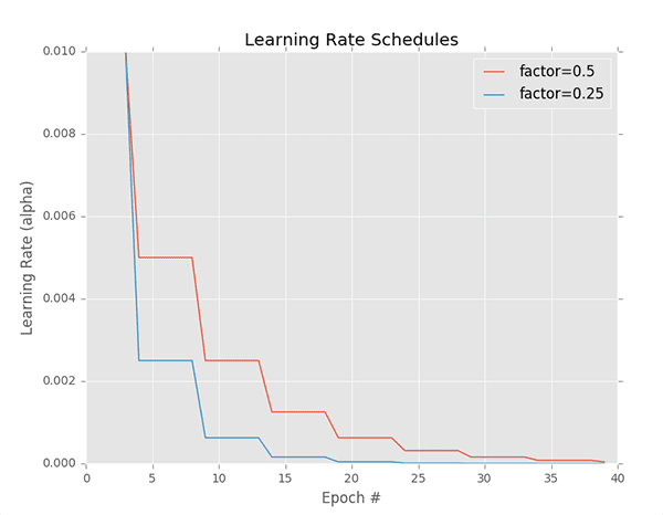
Figure 2: Keras learning rate step-based decay. The schedule in red is a decay factor of 0.5 and blue is a factor of 0.25.

One popular learning rate scheduler is step-based decay where we systematically drop the learning rate after specific epochs during training.

The step decay learning rate scheduler can be seen as a piecewise function, as visualized in Figure 2 — here the learning rate is constant for a number of epochs, then drops, is constant once more, then drops again, etc.

When applying step decay to our learning rate, we have two options:

Define an equation that models the piecewise drop-in learning rate that we wish to achieve.
Use what I call the
```
ctrl + c
```
method to train a deep neural network. Here we train for some number of epochs at a given learning rate and eventually notice validation performance stagnating/stalling, then
```
ctrl + c
```
to stop the script, adjust our learning rate, and continue training.

We’ll primarily be focusing on the equation-based piecewise drop to learning rate scheduling in this post.

The

ctrl + c

method is a bit more advanced and normally applied to larger datasets using deeper neural networks where the exact number of epochs required to obtain a reasonable model is unknown.

If you’d like to learn more about the

ctrl + c

method to training, please refer to Deep Learning for Computer Vision with Python.

When applying step decay, we often drop our learning rate by either (1) half or (2) an order of magnitude after every fixed number of epochs. For example, let’s suppose our initial learning rate is $\alpha = 0.01$ .

After 10 epochs we drop the learning rate to $\alpha = 0.005$ .

After another 10 epochs (i.e., the 20th total epoch), $\alpha$ is dropped by a factor of

0.5

again, such that $\alpha = 0.0025$ , etc.

In fact, this is the exact same learning rate schedule that is depicted in Figure 2 (red line).

The blue line displays a more aggressive drop factor of

0.25

. Modeled mathematically, we can define our step-based decay equation as: $\alpha_{E + 1} = \alpha_{I} \times F^{(1 + E) / D}$

Where $\alpha_{I}$ is the initial learning rate, is the factor value controlling the rate in which the learning date drops, D is the “Drop every” epochs value, and E is the current epoch.

The larger our factor is, the slower the learning rate will decay.

Conversely, the smaller the factor , the faster the learning rate will decay.

All that said, let’s go ahead and implement our

StepDecay

class now.

Go back to your

learning_rate_schedulers.py

file and insert the following code:

class StepDecay(LearningRateDecay):
	def __init__(self, initAlpha=0.01, factor=0.25, dropEvery=10):
		# store the base initial learning rate, drop factor, and
		# epochs to drop every
		self.initAlpha = initAlpha
		self.factor = factor
		self.dropEvery = dropEvery

	def __call__(self, epoch):
		# compute the learning rate for the current epoch
		exp = np.floor((1 + epoch) / self.dropEvery)
		alpha = self.initAlpha * (self.factor ** exp)

		# return the learning rate
		return float(alpha)

Line 20 defines the constructor to our

StepDecay

class. We then store the initial learning rate (

initAlpha

), drop factor, and

dropEvery

epochs values (Lines 23-25).

The

__call__

function:

Accepts the current
```
epoch
```
number.
Computes the learning rate based on the step-based decay formula detailed above (Lines 29 and 30).
Returns the computed learning rate for the current epoch (Line 33).

You’ll see how to use this learning rate schedule later in this post.

Linear and polynomial learning rate schedules in Keras

Two of my favorite learning rate schedules are linear learning rate decay and polynomial learning rate decay.

Using these methods our learning rate is decayed to zero over a fixed number of epochs.

The rate in which the learning rate is decayed is based on the parameters to the polynomial function. A smaller exponent/power to the polynomial will cause the learning rate to decay “more slowly”, whereas larger exponents decay the learning rate “more quickly”.

Conveniently, both of these methods can be implemented in a single class:

class PolynomialDecay(LearningRateDecay):
	def __init__(self, maxEpochs=100, initAlpha=0.01, power=1.0):
		# store the maximum number of epochs, base learning rate,
		# and power of the polynomial
		self.maxEpochs = maxEpochs
		self.initAlpha = initAlpha
		self.power = power

	def __call__(self, epoch):
		# compute the new learning rate based on polynomial decay
		decay = (1 - (epoch / float(self.maxEpochs))) ** self.power
		alpha = self.initAlpha * decay

		# return the new learning rate
		return float(alpha)

Line 36 defines the constructor to our

PolynomialDecay

class which requires three values:

```
maxEpochs
```
: The total number of epochs we’ll be training for.
```
initAlpha
```
: The initial learning rate.
```
power
```
: The power/exponent of the polynomial.

Note that if you set

power=1.0

then you have a linear learning rate decay.

Lines 45 and 46 compute the adjusted learning rate for the current epoch while Line 49 returns the new learning rate.

Implementing our training script

Now that we’ve implemented a few different Keras learning rate schedules, let’s see how we can use them inside an actual training script.

Create a file named

train.py

file in your editor and insert the following code:

# set the matplotlib backend so figures can be saved in the background
import matplotlib
matplotlib.use("Agg")

# import the necessary packages
from pyimagesearch.learning_rate_schedulers import StepDecay
from pyimagesearch.learning_rate_schedulers import PolynomialDecay
from pyimagesearch.resnet import ResNet
from sklearn.preprocessing import LabelBinarizer
from sklearn.metrics import classification_report
from keras.callbacks import LearningRateScheduler
from keras.optimizers import SGD
from keras.datasets import cifar10
import matplotlib.pyplot as plt
import numpy as np
import argparse

Lines 2-16 import required packages. Line 3 sets the

matplotlib

backend so that we can create plots as image files. Our most notable imports include:

```
StepDecay
```
: Our class which calculates and plots step-based learning rate decay.
```
PolynomialDecay
```
: The class we wrote to calculate polynomial-based learning rate decay.
```
ResNet
```
: Our Convolutional Neural Network implemented in Keras.
```
LearningRateScheduler
```
: A Keras callback. We’ll pass our learning rate
```
schedule
```
to this class which will be called as a callback at the completion of each epoch to calculate our learning rate.

Let’s move on and parse our command line arguments:

# construct the argument parser and parse the arguments
ap = argparse.ArgumentParser()
ap.add_argument("-s", "--schedule", type=str, default="",
	help="learning rate schedule method")
ap.add_argument("-e", "--epochs", type=int, default=100,
	help="# of epochs to train for")
ap.add_argument("-l", "--lr-plot", type=str, default="lr.png",
	help="path to output learning rate plot")
ap.add_argument("-t", "--train-plot", type=str, default="training.png",
	help="path to output training plot")
args = vars(ap.parse_args())

Our script accepts any of four command line arguments when the script is called via the terminal:

```
--schedule
```
: The learning rate schedule method. Valid options are “standard”, “step”, “linear”, “poly”. By default, no learning rate schedule will be used.
```
--epochs
```
: The number of epochs to train for (
```
default=100
```
).
```
--lr-plot
```
: The path to the output plot. I suggest overriding the
```
default
```
of
```
lr.png
```
with a more descriptive path + filename.
```
--train-plot
```
: The path to the output accuracy/loss training history plot. Again, I suggest a descriptive path + filename, otherwise
```
training.png
```
will be set by
```
default
```
.

With our imports and command line arguments in hand, now it’s time to initialize our learning rate schedule:

# store the number of epochs to train for in a convenience variable,
# then initialize the list of callbacks and learning rate scheduler
# to be used
epochs = args["epochs"]
callbacks = []
schedule = None

# check to see if step-based learning rate decay should be used
if args["schedule"] == "step":
	print("[INFO] using 'step-based' learning rate decay...")
	schedule = StepDecay(initAlpha=1e-1, factor=0.25, dropEvery=15)

# check to see if linear learning rate decay should should be used
elif args["schedule"] == "linear":
	print("[INFO] using 'linear' learning rate decay...")
	schedule = PolynomialDecay(maxEpochs=epochs, initAlpha=1e-1, power=1)

# check to see if a polynomial learning rate decay should be used
elif args["schedule"] == "poly":
	print("[INFO] using 'polynomial' learning rate decay...")
	schedule = PolynomialDecay(maxEpochs=epochs, initAlpha=1e-1, power=5)

# if the learning rate schedule is not empty, add it to the list of
# callbacks
if schedule is not None:
	callbacks = [LearningRateScheduler(schedule)]

Line 33 sets the number of

epochs

we will train for directly from the command line

args

variable. From there we’ll initialize our

callbacks

list and learning rate

schedule

(Lines 34 and 35).

Lines 38-50 then select the learning rate

schedule

args["schedule"]

contains a valid value:

```
"step"
```
: Initializes
```
StepDecay
```
.
```
"linear"
```
: Initializes
```
PolynomialDecay
```
with
```
power=1
```
indicating that a linear learning rate decay will be utilized.
```
"poly"
```
:
```
PolynomialDecay
```
with a
```
power=5
```
will be used.

After you’ve reproduced the results of the experiments in this tutorial, be sure to revisit Lines 38-50 and insert additional

elif

statements of your own so you can run some of your own experiments!

Lines 54 and 55 initialize the

LearningRateScheduler

with the schedule as a single callback part of the

callbacks

list. There is a case where no learning rate decay will be used (i.e. if the

--schedule

command line argument is not overridden when the script is executed).

Let’s go ahead and load our data:

# load the training and testing data, then scale it into the
# range [0, 1]
print("[INFO] loading CIFAR-10 data...")
((trainX, trainY), (testX, testY)) = cifar10.load_data()
trainX = trainX.astype("float") / 255.0
testX = testX.astype("float") / 255.0

# convert the labels from integers to vectors
lb = LabelBinarizer()
trainY = lb.fit_transform(trainY)
testY = lb.transform(testY)

# initialize the label names for the CIFAR-10 dataset
labelNames = ["airplane", "automobile", "bird", "cat", "deer",
	"dog", "frog", "horse", "ship", "truck"]

Line 60 loads our CIFAR-10 data. The dataset is conveniently already split into training and testing sets.

The only preprocessing we must perform is to scale the data into the range [0, 1] (Lines 61 and 62).

Lines 65-67 binarize the labels and then Lines 70 and 71 initialize our

labelNames

(i.e. classes). Do not add to or alter the

labelNames

list as order and length of the list matter.

Let’s initialize

decay

parameter:

# initialize the decay for the optimizer
decay = 0.0

# if we are using Keras' "standard" decay, then we need to set the
# decay parameter
if args["schedule"] == "standard":
	print("[INFO] using 'keras standard' learning rate decay...")
	decay = 1e-1 / epochs

# otherwise, no learning rate schedule is being used
elif schedule is None:
	print("[INFO] no learning rate schedule being used")

Line 74 initializes our learning rate

decay

If we’re using the

"standard"

learning rate decay schedule, then the decay is initialized as

1e-1 / epochs

(Lines 78-80).

With all of our initializations taken care of, let’s go ahead and compile + train our

ResNet

model:

# initialize our optimizer and model, then compile it
opt = SGD(lr=1e-1, momentum=0.9, decay=decay)
model = ResNet.build(32, 32, 3, 10, (9, 9, 9),
	(64, 64, 128, 256), reg=0.0005)
model.compile(loss="categorical_crossentropy", optimizer=opt,
	metrics=["accuracy"])

# train the network
H = model.fit(trainX, trainY, validation_data=(testX, testY),
	batch_size=128, epochs=epochs, callbacks=callbacks, verbose=1)

Our Stochastic Gradient Descent (

SGD

) optimizer is initialized on Line 87 using our

decay

From there, Lines 88 and 89 build our

ResNet

CNN with an input shape of 32x32x3 and 10 classes. For an in-depth review of ResNet, be sure refer to Chapter 10: ResNet of Deep Learning for Computer Vision with Python.

Our

model

is compiled with a

loss

function of

"categorical_crossentropy"

since our dataset has > 2 classes. If you use a different dataset with only 2 classes, be sure to use

loss="binary_crossentropy"

Lines 94 and 95 kick of our training process. Notice that we’ve provided the

callbacks

as a parameter. The

callbacks

will be called when each epoch is completed. Our

LearningRateScheduler

contained therein will handle our learning rate decay (so long as

callbacks

isn’t an empty list).

Finally, let’s evaluate our network and generate plots:

# evaluate the network
print("[INFO] evaluating network...")
predictions = model.predict(testX, batch_size=128)
print(classification_report(testY.argmax(axis=1),
	predictions.argmax(axis=1), target_names=labelNames))

# plot the training loss and accuracy
N = np.arange(0, args["epochs"])
plt.style.use("ggplot")
plt.figure()
plt.plot(N, H.history["loss"], label="train_loss")
plt.plot(N, H.history["val_loss"], label="val_loss")
plt.plot(N, H.history["acc"], label="train_acc")
plt.plot(N, H.history["val_acc"], label="val_acc")
plt.title("Training Loss and Accuracy on CIFAR-10")
plt.xlabel("Epoch #")
plt.ylabel("Loss/Accuracy")
plt.legend()
plt.savefig(args["train_plot"])

# if the learning rate schedule is not empty, then save the learning
# rate plot
if schedule is not None:
	schedule.plot(N)
	plt.savefig(args["lr_plot"])

Lines 99-101 evaluate our network and print a classification report to our terminal.

Lines 104-115 generate and save our training history plot (accuracy/loss curves). Lines 119-121 generate a learning rate schedule plot, if applicable. We will inspect these plot visualizations in the next section.

Keras learning rate schedule results

With both our (1) learning rate schedules and (2) training scripts implemented, let’s run some experiments to see which learning rate schedule will perform best given:

An initial learning rate of
```
1e-1
```
Training for a total of
```
100
```
epochs

Experiment #1: No learning rate decay/schedule

As a baseline, let’s first train our ResNet model on CIFAR-10 with no learning rate decay or schedule:

$ python train.py --train-plot output/train_no_schedule.png
[INFO] loading CIFAR-10 data...
[INFO] no learning rate being used
Train on 50000 samples, validate on 10000 samples
Epoch 1/100
50000/50000 [==============================] - 186s 4ms/step - loss: 2.1204 - acc: 0.4372 - val_loss: 1.9361 - val_acc: 0.5118
Epoch 2/100
50000/50000 [==============================] - 171s 3ms/step - loss: 1.5150 - acc: 0.6440 - val_loss: 1.5013 - val_acc: 0.6413
Epoch 3/100
50000/50000 [==============================] - 171s 3ms/step - loss: 1.2186 - acc: 0.7369 - val_loss: 1.2288 - val_acc: 0.7315
...
Epoch 98/100
50000/50000 [==============================] - 171s 3ms/step - loss: 0.5220 - acc: 0.9568 - val_loss: 1.0223 - val_acc: 0.8372
Epoch 99/100
50000/50000 [==============================] - 171s 3ms/step - loss: 0.5349 - acc: 0.9532 - val_loss: 1.0423 - val_acc: 0.8230
Epoch 100/100
50000/50000 [==============================] - 171s 3ms/step - loss: 0.5209 - acc: 0.9579 - val_loss: 0.9883 - val_acc: 0.8421
[INFO] evaluating network...
              precision    recall  f1-score   support

    airplane       0.84      0.86      0.85      1000
  automobile       0.90      0.93      0.92      1000
        bird       0.83      0.74      0.78      1000
         cat       0.67      0.79      0.73      1000
        deer       0.78      0.88      0.83      1000
         dog       0.85      0.69      0.76      1000
        frog       0.85      0.89      0.87      1000
       horse       0.94      0.82      0.88      1000
        ship       0.91      0.90      0.90      1000
       truck       0.90      0.90      0.90      1000

   micro avg       0.84      0.84      0.84     10000
   macro avg       0.85      0.84      0.84     10000
weighted avg       0.85      0.84      0.84     10000

Figure 3: Our first experiment for training ResNet on CIFAR-10 does not have learning rate decay.

Here we obtain ~85% accuracy, but as we can see, validation loss and accuracy stagnate past epoch ~15 and do not improve over the rest of the 100 epochs.

Our goal is now to utilize learning rate scheduling to beat our 85% accuracy (without overfitting).

Experiment: #2: Keras standard optimizer learning rate decay

In our second experiment we are going to use Keras’ standard decay-based learning rate schedule:

$ python train.py --schedule standard --train-plot output/train_standard_schedule.png
[INFO] loading CIFAR-10 data...
[INFO] using 'keras standard' learning rate decay...
Train on 50000 samples, validate on 10000 samples
Epoch 1/100
50000/50000 [==============================] - 184s 4ms/step - loss: 2.1074 - acc: 0.4460 - val_loss: 1.8397 - val_acc: 0.5334
Epoch 2/100
50000/50000 [==============================] - 171s 3ms/step - loss: 1.5068 - acc: 0.6516 - val_loss: 1.5099 - val_acc: 0.6663
Epoch 3/100
50000/50000 [==============================] - 171s 3ms/step - loss: 1.2097 - acc: 0.7512 - val_loss: 1.2928 - val_acc: 0.7176
...
Epoch 98/100
50000/50000 [==============================] - 171s 3ms/step - loss: 0.1752 - acc: 1.0000 - val_loss: 0.8892 - val_acc: 0.8209
Epoch 99/100
50000/50000 [==============================] - 171s 3ms/step - loss: 0.1746 - acc: 1.0000 - val_loss: 0.8923 - val_acc: 0.8204
Epoch 100/100
50000/50000 [==============================] - 171s 3ms/step - loss: 0.1740 - acc: 1.0000 - val_loss: 0.8924 - val_acc: 0.8208
[INFO] evaluating network...
              precision    recall  f1-score   support

    airplane       0.81      0.86      0.84      1000
  automobile       0.91      0.91      0.91      1000
        bird       0.75      0.71      0.73      1000
         cat       0.68      0.65      0.66      1000
        deer       0.78      0.81      0.79      1000
         dog       0.77      0.74      0.75      1000
        frog       0.83      0.88      0.85      1000
       horse       0.86      0.87      0.86      1000
        ship       0.90      0.90      0.90      1000
       truck       0.90      0.88      0.89      1000

   micro avg       0.82      0.82      0.82     10000
   macro avg       0.82      0.82      0.82     10000
weighted avg       0.82      0.82      0.82     10000

Figure 4: Our second learning rate decay schedule experiment uses Keras’ standard learning rate decay schedule.

This time we only obtain 82% accuracy, which goes to show, learning rate decay/scheduling will not always improve your results! You need to be careful which learning rate schedule you utilize.

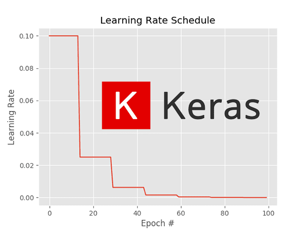
Experiment #3: Step-based learning rate schedule results

Let’s go ahead and perform step-based learning rate scheduling which will drop our learning rate by a factor of 0.25 every 15 epochs:

$ python train.py --schedule step --lr-plot output/lr_step_schedule.png --train-plot output/train_step_schedule.png
[INFO] using 'step-based' learning rate decay...
[INFO] loading CIFAR-10 data...
Train on 50000 samples, validate on 10000 samples
Epoch 1/100
50000/50000 [==============================] - 186s 4ms/step - loss: 2.2839 - acc: 0.4328 - val_loss: 1.8936 - val_acc: 0.5530
Epoch 2/100
50000/50000 [==============================] - 171s 3ms/step - loss: 1.6425 - acc: 0.6213 - val_loss: 1.4599 - val_acc: 0.6749
Epoch 3/100
50000/50000 [==============================] - 171s 3ms/step - loss: 1.2971 - acc: 0.7177 - val_loss: 1.3298 - val_acc: 0.6953
...
Epoch 98/100
50000/50000 [==============================] - 171s 3ms/step - loss: 0.1817 - acc: 1.0000 - val_loss: 0.7221 - val_acc: 0.8653
Epoch 99/100
50000/50000 [==============================] - 171s 3ms/step - loss: 0.1817 - acc: 1.0000 - val_loss: 0.7228 - val_acc: 0.8661
Epoch 100/100
50000/50000 [==============================] - 171s 3ms/step - loss: 0.1817 - acc: 1.0000 - val_loss: 0.7267 - val_acc: 0.8652
[INFO] evaluating network...
              precision    recall  f1-score   support

    airplane       0.86      0.89      0.87      1000
  automobile       0.94      0.93      0.94      1000
        bird       0.83      0.80      0.81      1000
         cat       0.75      0.73      0.74      1000
        deer       0.82      0.87      0.84      1000
         dog       0.82      0.77      0.79      1000
        frog       0.89      0.90      0.90      1000
       horse       0.91      0.90      0.90      1000
        ship       0.93      0.93      0.93      1000
       truck       0.90      0.93      0.92      1000

   micro avg       0.87      0.87      0.87     10000
   macro avg       0.86      0.87      0.86     10000
weighted avg       0.86      0.87      0.86     10000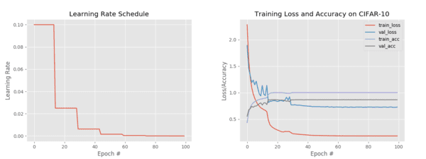

Figure 5: Experiment #3 demonstrates a step-based learning rate schedule (left). The training history accuracy/loss curves are shown on the right.

Figure 5 (left) visualizes our learning rate schedule. Notice how after every 15 epochs our learning rate drops, creating the “stair-step”-like effect.

Figure 5 (right) demonstrates the classic signs of step-based learning rate scheduling — you can clearly see our:

Training/validation loss decrease
Training/validation accuracy increase

…when our learning rate is dropped.

This is especially pronounced in the first two drops (epochs 15 and 30), after which the drops become less substantial.

This type of steep drop is a classic sign of a step-based learning rate schedule being utilized — if you see that type of training behavior in a paper, publication, or another tutorial, you can be almost sure that they used step-based decay!

Getting back to our accuracy, we’re now at 86-87% accuracy, an improvement from our first experiment.

Experiment #4: Linear learning rate schedule results

Let’s try using a linear learning rate schedule with Keras by setting

power=1.0

$ python train.py --schedule linear --lr-plot output/lr_linear_schedule.png --train-plot output/train_linear_schedule.png
[INFO] using 'linear' learning rate decay...
[INFO] loading CIFAR-10 data...
Epoch 1/100
50000/50000 [==============================] - 187s 4ms/step - loss: 2.0399 - acc: 0.4541 - val_loss: 1.6900 - val_acc: 0.5789
Epoch 2/100
50000/50000 [==============================] - 171s 3ms/step - loss: 1.4623 - acc: 0.6588 - val_loss: 1.4535 - val_acc: 0.6557
Epoch 3/100
50000/50000 [==============================] - 171s 3ms/step - loss: 1.1790 - acc: 0.7480 - val_loss: 1.2633 - val_acc: 0.7230
...
Epoch 98/100
50000/50000 [==============================] - 171s 3ms/step - loss: 0.1025 - acc: 1.0000 - val_loss: 0.5623 - val_acc: 0.8804
Epoch 99/100
50000/50000 [==============================] - 171s 3ms/step - loss: 0.1021 - acc: 1.0000 - val_loss: 0.5636 - val_acc: 0.8800
Epoch 100/100
50000/50000 [==============================] - 171s 3ms/step - loss: 0.1019 - acc: 1.0000 - val_loss: 0.5622 - val_acc: 0.8808
[INFO] evaluating network...
              precision    recall  f1-score   support

    airplane       0.88      0.91      0.89      1000
  automobile       0.94      0.94      0.94      1000
        bird       0.84      0.81      0.82      1000
         cat       0.78      0.76      0.77      1000
        deer       0.86      0.90      0.88      1000
         dog       0.84      0.80      0.82      1000
        frog       0.90      0.92      0.91      1000
       horse       0.91      0.91      0.91      1000
        ship       0.93      0.94      0.93      1000
       truck       0.93      0.93      0.93      1000

   micro avg       0.88      0.88      0.88     10000
   macro avg       0.88      0.88      0.88     10000
weighted avg       0.88      0.88      0.88     10000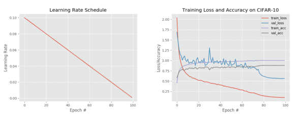

Figure 6: Linear learning rate decay (left) applied to ResNet on CIFAR-10 over 100 epochs with Keras. The training accuracy/loss curve is displayed on the right.

Figure 6 (left) shows that our learning rate is decreasing linearly over time while Figure 6 (right) visualizes our training history.

We’re now seeing a sharper drop in both training and validation loss, especially past approximately epoch 75; however, note that our training loss is dropping significantly faster than our validation loss — we may be at risk of overfitting.

Regardless, we are now obtaining 88% accuracy on our data, our best result thus far.

Experiment #5: Polynomial learning rate schedule results

As a final experiment let’s apply polynomial learning rate scheduling with Keras by setting

power=5

$ python train.py --schedule poly --lr-plot output/lr_poly_schedule.png --train-plot output/train_poly_schedule.png
[INFO] using 'polynomial' learning rate decay...
[INFO] loading CIFAR-10 data...
Epoch 1/100
50000/50000 [==============================] - 186s 4ms/step - loss: 2.0470 - acc: 0.4445 - val_loss: 1.7379 - val_acc: 0.5576
Epoch 2/100
50000/50000 [==============================] - 171s 3ms/step - loss: 1.4793 - acc: 0.6448 - val_loss: 1.4536 - val_acc: 0.6513
Epoch 3/100
50000/50000 [==============================] - 171s 3ms/step - loss: 1.2080 - acc: 0.7332 - val_loss: 1.2363 - val_acc: 0.7183
...
Epoch 98/100
50000/50000 [==============================] - 171s 3ms/step - loss: 0.1547 - acc: 1.0000 - val_loss: 0.6960 - val_acc: 0.8581
Epoch 99/100
50000/50000 [==============================] - 171s 3ms/step - loss: 0.1547 - acc: 1.0000 - val_loss: 0.6883 - val_acc: 0.8596
Epoch 100/100
50000/50000 [==============================] - 171s 3ms/step - loss: 0.1548 - acc: 1.0000 - val_loss: 0.6942 - val_acc: 0.8601
[INFO] evaluating network...
              precision    recall  f1-score   support

    airplane       0.86      0.89      0.87      1000
  automobile       0.94      0.94      0.94      1000
        bird       0.78      0.80      0.79      1000
         cat       0.75      0.70      0.73      1000
        deer       0.83      0.86      0.84      1000
         dog       0.81      0.78      0.79      1000
        frog       0.86      0.91      0.89      1000
       horse       0.92      0.88      0.90      1000
        ship       0.94      0.92      0.93      1000
       truck       0.91      0.92      0.91      1000

   micro avg       0.86      0.86      0.86     10000
   macro avg       0.86      0.86      0.86     10000
weighted avg       0.86      0.86      0.86     10000

Figure 7: Polynomial-based learning decay results using Keras.

Figure 7 (left) visualizes the fact that our learning rate is now decaying according to our polynomial function while Figure 7 (right) plots our training history.

This time we obtain ~86% accuracy.

Commentary on learning rate schedule experiments

Our best experiment was from our fourth experiment where we utilized a linear learning rate schedule.

But does that mean we should always use a linear learning rate schedule?

No, far from it, actually.

The key takeaway here is that for this:

Particular dataset (CIFAR-10)
Particular neural network architecture (ResNet)
Initial learning rate of 1e-2
Number of training epochs (100)

…is that linear learning rate scheduling worked the best.

No two deep learning projects are alike so you will need to run your own set of experiments, including varying the initial learning rate and the total number of epochs, to determine the appropriate learning rate schedule (additional commentary is included in the “Summary” section of this tutorial as well).

Do other learning rate schedules exist?

Other learning rate schedules exist, and in fact, any mathematical function that can accept an epoch or batch number as an input and returns a learning rate can be considered a “learning rate schedule”. Two other learning rate schedules you may encounter include (1) exponential learning rate decay, as well as (2) cyclical learning rates.

I don’t often use exponential decay as I find that linear and polynomial decay are more than sufficient, but you are more than welcome to subclass the

LearningRateDecay

class and implement exponential decay if you so wish.

Cyclical learning rates, on the other hand, are very powerful — we’ll be covering cyclical learning rates in a tutorial later in this series.

How do I choose my initial learning rate?

You’ll notice that in this tutorial we did not vary our learning rate, we kept it constant at

1e-2

When performing your own experiments you’ll want to combine:

Learning rate schedules…
…with different learning rates

Don’t be afraid to mix and match!

The four most important hyperparameters you’ll want to explore, include:

Initial learning rate
Number of training epochs
Learning rate schedule
Regularization strength/amount (L2, dropout, etc.)

Finding an appropriate balance of each can be challenging, but through many experiments, you’ll be able to find a recipe that leads to a highly accurate neural network.

If you’d like to learn more about my tips, suggestions, and best practices for learning rates, learning rate schedules, and training your own neural networks, refer to my book, Deep Learning for Computer Vision with Python.

Where can I learn more?

Figure 8: Deep Learning for Computer Vision with Python is a deep learning book for beginners, practitioners, and experts alike.

Today’s tutorial introduced you to learning rate decay and schedulers using Keras. To learn more about learning rates, schedulers, and how to write custom callback functions, refer to my book, Deep Learning for Computer Vision with Python.

Inside the book I cover:

More details on learning rates (and how a solid understanding of the concept impacts your deep learning success)
How to spot under/overfitting on-the-fly with a custom training monitor callback
How to checkpoint your models with a custom callback
My tips/tricks, suggestions, and best practices for training CNNs

Besides content on learning rates, you’ll also find:

Super practical walkthroughs that present solutions to actual, real-world image classification, object detection, and instance segmentation problems.
Hands-on tutorials (with lots of code) that not only show you the algorithms behind deep learning for computer vision but their implementations as well.
A no-nonsense teaching style that is guaranteed to help you master deep learning for image understanding and visual recognition.

To learn more about the book, and grab the table of contents + free sample chapters, just click here!

Grab my free sample chapters!

Summary

In this tutorial, you learned how to utilize Keras for learning rate decay and learning rate scheduling.

Specifically, you discovered how to implement and utilize a number of learning rate schedules with Keras, including:

The decay schedule built into most Keras optimizers
Step-based learning rate schedules
Linear learning rate decay
Polynomial learning rate schedules

After implementing our learning rate schedules we evaluated each on a set of experiments on the CIFAR-10 dataset.

Our results demonstrated that for an initial learning rate of

1e-2

, the linear learning rate schedule, decaying over

epochs, performed the best.

However, this does not mean that a linear learning rate schedule will always outperform other types of schedules. Instead, all this means is that for this:

Particular dataset (CIFAR-10)
Particular neural network architecture (ResNet)
Initial learning rate of
```
1e-2
```
Number of training epochs (
```
100
```
)

…that linear learning rate scheduling worked the best.

No two deep learning projects are alike so you will need to run your own set of experiments, including varying the initial learning rate, to determine the appropriate learning rate schedule.

I suggest you keep an experiment log that details any hyperparameter choices and associated results, that way you can refer back to it and double-down on experiments that look promising.

Do not expect that you’ll be able to train a neural network and be “one and done” — that rarely, if ever, happens. Instead, set the expectation with yourself that you’ll be running many experiments and tuning hyperparameters as you go along. Machine learning, deep learning, and artificial intelligence as a whole are iterative — you build on your previous results.

Later in this series of tutorials I’ll also be showing you how to select your initial learning rate.

To download the source code to this post, and be notified when future tutorials are published here on PyImageSearch, just enter your email address in the form below!

Downloads:

The post Keras learning rate schedules and decay appeared first on PyImageSearch.

Keras learning rate schedules and decay

Why adjust our learning rate and use learning rate schedules?

Project structure

The standard “decay” schedule in Keras

Our LearningRateDecay class

Step-based learning rate schedules with Keras

Linear and polynomial learning rate schedules in Keras

Implementing our training script

Keras learning rate schedule results

Experiment #1: No learning rate decay/schedule

Experiment: #2: Keras standard optimizer learning rate decay

Experiment #3: Step-based learning rate schedule results

Experiment #4: Linear learning rate schedule results

Experiment #5: Polynomial learning rate schedule results

Commentary on learning rate schedule experiments

Do other learning rate schedules exist?

How do I choose my initial learning rate?

Where can I learn more?

Summary

Downloads:

Trending Articles

Our `LearningRateDecay` class